"Labels are expensive, but data has structure for free. You just have to teach the model to notice."
A Pretext Task With Existential Purpose
Supervised learning requires labels. In scientific domains, labels are scarce: annotating protein functions costs months of wet-lab work, classifying astronomical transients requires expert review, and labeling medical images demands board-certified specialists. Self-supervised learning (SSL) sidesteps this bottleneck entirely by extracting supervision from the structure of the data itself. A model learns to predict masked tokens, distinguish augmented views of the same sample, or reconstruct corrupted inputs. The resulting encoder captures deep structural patterns that transfer to downstream tasks with minimal labeled data. This section covers the three SSL paradigms (masked prediction, contrastive learning, generative modeling), explains why each works, and shows how to implement them in PyTorch.
1. The Label Bottleneck in Science
Consider the challenge facing a materials scientist studying metal-organic frameworks (MOFs). There are millions of possible MOF structures, each characterized by its crystal geometry, pore topology, and chemical composition. To predict which MOFs adsorb CO2 efficiently, a researcher would traditionally synthesize candidates, measure adsorption isotherms, and train a supervised model on the labeled data. But synthesis and measurement are slow. A year of intensive work might yield 10,000 labeled examples, while the space of possible structures remains combinatorially vast.
Self-supervised learning offers an alternative path. Instead of predicting a labeled property, we train an encoder to understand the structure of MOFs from millions of unlabeled crystal descriptions. The encoder learns what makes a valid MOF, how pore geometry relates to framework topology, and which chemical motifs tend to co-occur. This structural knowledge, captured as a vector representation, transfers to downstream property prediction with far fewer labeled examples than training from scratch would require.
Without self-supervised pretraining, a protein function predictor trained on 500 labeled examples typically learns very little (as observed in benchmarks such as TAPE and PEER); with it, the same 500 labels can yield accuracy that rivals models trained on 100 times more supervised data. That gap between success and failure hinges on a single idea.
What. Self-supervised learning is a family of methods that create supervised learning tasks from unlabeled data by exploiting structure, redundancy, or co-occurrence patterns within the data itself.
Common Misconception
A frequent misunderstanding is that self-supervised learning uses no supervision at all. In reality, SSL generates its own supervision signal automatically from the data: for example, the original unmasked token serves as the label for a masked prediction task. The "self" in self-supervised refers to the fact that the training signal comes from the data's own structure rather than from human-provided annotations, not that the model trains without any objective to optimize.
Why. In science, labeled data is the bottleneck. Unlabeled data is abundant: millions of protein sequences in UniProt, billions of molecular structures in PubChem, petabytes of astronomical survey images. SSL converts this abundance into powerful pretrained encoders.
How. By defining a pretext task, where a pretext task is an auxiliary objective whose labels are derived automatically from the data's own structure, requiring the model to learn useful features as a byproduct of solving it. Examples include predicting masked portions of the input, distinguishing real data from corrupted versions, or reconstructing inputs from compressed representations.
When. When labeled data is scarce relative to the complexity of the task, when unlabeled data is abundant, and when the domain has rich internal structure (most scientific domains qualify on all three counts). In short: teach a model to finish the sentence, and it will learn the language; teach it the language, and the labels barely matter.
A pretext task works because solving it requires learning features that are also useful for downstream tasks. Predicting masked amino acids in a protein sequence forces the model to learn evolutionary conservation patterns, secondary structure preferences, and co-evolutionary constraints. These are exactly the features a biologist would want for function prediction, stability estimation, or variant effect classification. The pretext task provides no explicit labels about function; the useful features emerge as a side effect of learning to solve the self-supervised objective. The art of SSL is choosing pretext tasks whose solutions require the right kind of understanding.
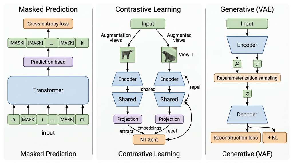
The three SSL paradigms each extract supervision differently, as Figure 26.1 illustrates. Masked prediction hides part of the input and reconstructs it. Contrastive learning pulls similar pairs together and pushes dissimilar pairs apart. Generative modeling compresses inputs into a latent space and reconstructs them through a decoder.
2. Paradigm 1: Masked Prediction
Masked prediction is the simplest and most intuitive SSL paradigm. The idea: hide part of the input, then train the model to reconstruct the hidden part from the visible context. If the model can fill in the blanks, it must have learned the statistical structure of the data.
In masked prediction, a fraction of input elements (tokens, pixels, graph nodes) are replaced with a placeholder. The model then learns to recover the original values using only the surrounding context. It matters because it converts any large corpus of sequential or structured data into a virtually unlimited source of training examples, with no human labeling required. A neural network (typically a transformer) reads the corrupted input and outputs a probability distribution over possible original values at each masked position. Cross-entropy loss drives the optimization. Prefer masked prediction over contrastive learning when the data has strong local dependencies (sequences, grids, graphs) and you need contextual, per-position representations rather than a single global embedding. Choose contrastive methods instead when the goal is a holistic similarity metric and you can design meaningful augmentations.
The approach was popularized by BERT (Bidirectional Encoder Representations from Transformers), which masks 15% of tokens in a text sequence and trains a transformer to predict them. The same principle applies far beyond text. Masked autoencoders (MAE) mask random patches of images. ESM-2 masks amino acids in protein sequences. Masked graph neural networks mask nodes or edges in molecular graphs. The same idea applies to Simplified Molecular Input Line Entry System (SMILES) strings, spectra, and other structured scientific data.
The masked prediction objective for a sequence \(x = (x_1, x_2, \ldots, x_n)\) with masked positions \(\mathcal{M} \subset \{1, \ldots, n\}\) is:
$$\mathcal{L}_{\text{mask}} = -\sum_{i \in \mathcal{M}} \log p_\theta(x_i \mid x_{\setminus \mathcal{M}})$$where \(x_{\setminus \mathcal{M}}\) denotes the input with masked positions replaced by a special token, and \(p_\theta\) is the model's predicted distribution over possible values at each masked position.
The following listing implements masked prediction for a simple sequence encoder.
import torch
import torch.nn as nn
import torch.nn.functional as F

class MaskedSequenceEncoder(nn.Module):
    """Transformer encoder trained with masked token prediction."""

    def __init__(self, vocab_size: int, d_model: int = 256,
                 nhead: int = 8, num_layers: int = 4,
                 mask_ratio: float = 0.15):
        super().__init__()
        self.mask_ratio = mask_ratio
        self.mask_token_id = vocab_size  # dedicated mask token

        self.embedding = nn.Embedding(vocab_size + 1, d_model)  # +1 for mask
        self.pos_encoding = nn.Embedding(512, d_model)

        encoder_layer = nn.TransformerEncoderLayer(
            d_model=d_model, nhead=nhead, dim_feedforward=4 * d_model,
            batch_first=True, norm_first=True
        )
        self.transformer = nn.TransformerEncoder(
            encoder_layer, num_layers=num_layers
        )
        # Prediction head: project back to vocabulary
        self.pred_head = nn.Linear(d_model, vocab_size)

    def mask_input(self, tokens: torch.Tensor):
        """Apply random masking. Returns masked input and targets."""
        mask = torch.rand_like(tokens.float()) < self.mask_ratio
        masked_tokens = tokens.clone()
        masked_tokens[mask] = self.mask_token_id
        return masked_tokens, mask

    def encode(self, tokens: torch.Tensor) -> torch.Tensor:
        """Produce representations (no masking, for downstream use)."""
        positions = torch.arange(tokens.size(1), device=tokens.device)
        x = self.embedding(tokens) + self.pos_encoding(positions)
        return self.transformer(x)

    def forward(self, tokens: torch.Tensor):
        """Forward pass with masking for training."""
        masked_tokens, mask = self.mask_input(tokens)
        positions = torch.arange(tokens.size(1), device=tokens.device)
        x = self.embedding(masked_tokens) + self.pos_encoding(positions)
        h = self.transformer(x)
        logits = self.pred_head(h)  # (batch, seq_len, vocab_size)
        return logits, mask

def masked_prediction_loss(logits, targets, mask):
    """Compute cross-entropy only at masked positions."""
    masked_logits = logits[mask]     # (num_masked, vocab_size)
    masked_targets = targets[mask]   # (num_masked,)
    return F.cross_entropy(masked_logits, masked_targets)

# Training loop sketch
vocab_size = 25  # e.g., 20 amino acids + 5 special tokens
model = MaskedSequenceEncoder(vocab_size, d_model=128, num_layers=2)
optimizer = torch.optim.AdamW(model.parameters(), lr=1e-4)

# Simulate a batch of protein-like sequences
batch = torch.randint(0, 20, (32, 64))  # 32 sequences, length 64

for step in range(100):
    logits, mask = model(batch)
    loss = masked_prediction_loss(logits, batch, mask)
    optimizer.zero_grad()
    loss.backward()
    optimizer.step()
    if step % 20 == 0:
        accuracy = (logits[mask].argmax(-1) == batch[mask]).float().mean()
        print(f"Step {step}: loss={loss.item():.3f}, "
f"mask_acc={accuracy.item():.3f}")encode method produces representations for downstream use without masking.Researchers at MIT applied masked prediction to SMILES strings (text representations of molecules). By training a transformer to predict masked atoms and bonds in millions of SMILES from PubChem, they learned representations that captured chemical structure without any property labels. The pretrained encoder achieved competitive or state-of-the-art results on several molecular property prediction benchmarks (MoleculeNet) at the time of publication after fine-tuning with just a few hundred labeled examples per task. The model learned, for instance, that carbon atoms bonded to electronegative groups tend to be electrophilic, that aromatic rings prefer planar geometries, and that certain functional groups (hydroxyl, carboxyl) co-occur in drug-like molecules. None of this chemistry was explicitly labeled; it emerged from the statistics of valid SMILES strings.
3. Paradigm 2: Contrastive Learning
Contrastive learning takes a fundamentally different approach: instead of reconstructing inputs, it learns to distinguish similar inputs from dissimilar ones. Given an anchor sample, the model should produce representations that are close to representations of semantically related samples (positives) and far from representations of unrelated samples (negatives).
Mental Model
Think of contrastive learning as a wine tasting exercise. You are given three glasses: two contain the same wine poured from the same bottle (the positive pair) and one contains a different wine (the negative). Your task is to identify which two match. To succeed, you must learn to focus on the features that define a wine's identity (grape varietal, tannin profile, acidity) while ignoring superficial differences between the two pours of the same wine (slight temperature variation, different glass shape). Over hundreds of such tastings with many different wines, you develop a refined palate that captures the deep characteristics of any wine in a compact mental profile. Contrastive learning works the same way: by repeatedly asking the model "which two are the same?", it learns to encode the features that define identity while discarding the variations introduced by augmentation.
The critical design choice is how to define "similar" without labels. The most common strategy is augmentation invariance (the principle that a model's representation should not change when the input is transformed in ways that preserve its meaning): two different augmentations of the same input are positives, while augmentations of different inputs are negatives. For images, augmentations include random cropping, color jitter, and Gaussian blur. For text, they include dropout masks, back-translation, or sentence reordering. For molecules, they might include subgraph sampling or atom masking.
The contrastive objective pulls positive pairs together and pushes negative pairs apart in embedding space. Section 26.2 develops the mathematical details; the focus here is the conceptual framework and the three major architectures.
SimCLR: Simplicity Through Scale
SimCLR (Simple Framework for Contrastive Learning of Visual Representations) takes the most direct approach. Given a batch of \(N\) samples, create two augmented views of each, producing \(2N\) views total. Pass all views through an encoder \(f\) and a projection head \(g\), where a projection head is a small neural network (typically a two-layer MLP) that maps encoder output to a lower-dimensional space optimized for the contrastive objective. For each sample, the two views of that sample form the positive pair; the remaining \(2(N-1)\) views are negatives. The training signal comes from the NT-Xent loss (normalized temperature-scaled cross-entropy), which we derive formally in Section 26.2.
import torch
import torch.nn as nn
import torch.nn.functional as F

class SimCLR(nn.Module):
    """SimCLR: contrastive learning with augmented pairs."""

    def __init__(self, encoder: nn.Module, feature_dim: int,
                 proj_dim: int = 128, temperature: float = 0.07):
        super().__init__()
        self.encoder = encoder
        self.temperature = temperature

        # Projection head: maps encoder features to contrastive space
        self.projector = nn.Sequential(
            nn.Linear(feature_dim, feature_dim),
            nn.ReLU(),
            nn.Linear(feature_dim, proj_dim)
        )

    def forward(self, x1: torch.Tensor, x2: torch.Tensor):
        """Compute NT-Xent loss for two augmented views.

        Args:
            x1, x2: Two augmented views, each (batch_size, ...).
        Returns:
            loss: Scalar NT-Xent loss.
        """
        # Encode both views
        h1 = self.encoder(x1)  # (N, feature_dim)
        h2 = self.encoder(x2)  # (N, feature_dim)

        # Project to contrastive space
        z1 = F.normalize(self.projector(h1), dim=1)  # (N, proj_dim)
        z2 = F.normalize(self.projector(h2), dim=1)  # (N, proj_dim)

        N = z1.size(0)
        z = torch.cat([z1, z2], dim=0)  # (2N, proj_dim)

        # Cosine similarity matrix
        sim = torch.mm(z, z.t()) / self.temperature  # (2N, 2N)

        # Mask out self-similarity (diagonal)
        mask = ~torch.eye(2 * N, dtype=torch.bool, device=z.device)
        sim = sim.masked_fill(~mask, float('-inf'))

        # Positive pairs: (i, i+N) and (i+N, i)
        labels = torch.cat([
            torch.arange(N, 2 * N, device=z.device),  # view1 -> view2
            torch.arange(0, N, device=z.device)        # view2 -> view1
        ])

        loss = F.cross_entropy(sim, labels)
        return loss

# Example: SimCLR with a simple multilayer perceptron (MLP) encoder on tabular data
encoder = nn.Sequential(
    nn.Linear(128, 256), nn.ReLU(),
    nn.Linear(256, 256), nn.ReLU(),
    nn.Linear(256, 128)
)
model = SimCLR(encoder, feature_dim=128, proj_dim=64)

# Simulate augmented pair batch (e.g., dropout noise as augmentation)
x1 = F.dropout(torch.randn(64, 128), p=0.1)
x2 = F.dropout(torch.randn(64, 128), p=0.1)
loss = model(x1, x2)
print(f"NT-Xent loss: {loss.item():.4f}")MoCo: Momentum Contrast
SimCLR's effectiveness depends on large batch sizes (4096 or more in the original paper) because each batch provides the negative samples. MoCo (Momentum Contrast) decouples the negative set from the batch size by maintaining a queue of recent representations from a momentum-updated encoder.
The key idea: keep two encoders, a query encoder \(f_q\) (updated by gradient descent) and a key encoder \(f_k\) (updated as an exponential moving average of \(f_q\), meaning each parameter of \(f_k\) is slowly blended toward the corresponding parameter of \(f_q\) after every training step). The query encoder processes the current batch; the key encoder populates a first-in-first-out (FIFO) queue of negatives. This lets you use 65,536 negatives regardless of batch size.
The momentum update rule is: \(\theta_k \leftarrow m \cdot \theta_k + (1 - m) \cdot \theta_q\), with \(m = 0.999\) being the typical momentum coefficient. The slow update ensures the keys in the queue are approximately consistent, produced by encoders that differ only slightly.
class MoCo(nn.Module):
    """Momentum Contrast with a dictionary queue."""

    def __init__(self, encoder_fn, feature_dim: int, proj_dim: int = 128,
                 queue_size: int = 65536, momentum: float = 0.999,
                 temperature: float = 0.07):
        super().__init__()
        self.queue_size = queue_size
        self.momentum = momentum
        self.temperature = temperature

        # Query encoder (updated by backprop)
        self.encoder_q = encoder_fn()
        self.projector_q = nn.Sequential(
            nn.Linear(feature_dim, feature_dim), nn.ReLU(),
            nn.Linear(feature_dim, proj_dim)
        )

        # Key encoder (momentum-updated copy)
        self.encoder_k = encoder_fn()
        self.projector_k = nn.Sequential(
            nn.Linear(feature_dim, feature_dim), nn.ReLU(),
            nn.Linear(feature_dim, proj_dim)
        )
        # Initialize key encoder with query encoder weights
        for param_q, param_k in zip(
            list(self.encoder_q.parameters())
            + list(self.projector_q.parameters()),
            list(self.encoder_k.parameters())
            + list(self.projector_k.parameters())
        ):
            param_k.data.copy_(param_q.data)
            param_k.requires_grad = False

        # Queue of negative keys
        self.register_buffer("queue", F.normalize(
            torch.randn(proj_dim, queue_size), dim=0
        ))
        self.register_buffer("queue_ptr",
                             torch.zeros(1, dtype=torch.long))

    @torch.no_grad()
    def _momentum_update(self):
        """Update key encoder as EMA of query encoder."""
        for param_q, param_k in zip(
            list(self.encoder_q.parameters())
            + list(self.projector_q.parameters()),
            list(self.encoder_k.parameters())
            + list(self.projector_k.parameters())
        ):
            param_k.data = (self.momentum * param_k.data
                           + (1.0 - self.momentum) * param_q.data)

    @torch.no_grad()
    def _enqueue(self, keys: torch.Tensor):
        """Add new keys to the queue, removing oldest entries."""
        batch_size = keys.size(0)
        ptr = int(self.queue_ptr)
        self.queue[:, ptr:ptr + batch_size] = keys.T
        self.queue_ptr[0] = (ptr + batch_size) % self.queue_size

    def forward(self, x_q: torch.Tensor, x_k: torch.Tensor):
        """Compute MoCo contrastive loss."""
        # Query representations
        q = F.normalize(
            self.projector_q(self.encoder_q(x_q)), dim=1
        )

        # Key representations (no gradient)
        with torch.no_grad():
            self._momentum_update()
            k = F.normalize(
                self.projector_k(self.encoder_k(x_k)), dim=1
            )

        # Positive logits: (N, 1)
        pos = (torch.einsum('nc,nc->n', q, k).unsqueeze(1)
               / self.temperature)
        # Negative logits: (N, queue_size)
        neg = torch.mm(q, self.queue.clone().detach()) / self.temperature

        # Logits: positives first, then negatives
        logits = torch.cat([pos, neg], dim=1)
        labels = torch.zeros(logits.size(0), dtype=torch.long,
                            device=logits.device)

        loss = F.cross_entropy(logits, labels)
        self._enqueue(k)
return lossCLIP: Cross-Modal Contrastive Learning
Both SimCLR and MoCo learn by contrasting augmented views within a single modality, but the same principle of pulling matching pairs together applies equally well when the two views come from entirely different data types.
CLIP (Contrastive Language-Image Pretraining) extends contrastive learning across modalities: instead of two augmented views of the same image, the positive pair is an image and its caption. The model learns a shared embedding space where semantically matching images and texts are close together. This enables remarkable zero-shot capabilities: to classify images, describe each class in text, embed both image and text descriptions, and pick the closest text embedding.
For scientific discovery, the CLIP paradigm is powerful: align molecular structures with textual descriptions of properties, electron microscopy images with materials specifications, or spectra with compound identities. Chapter 28 covers multimodal alignment in depth.
The SSL revolution has spread far beyond its origins in computer vision and NLP. ESM-2 (Lin et al., 2023) used masked prediction on 250 million protein sequences; ESMFold, built on ESM-2 embeddings, became the fastest competitive protein structure predictor after AlphaFold. GNoME (2023) combined graph neural network pretraining on crystal structures with active learning and DFT validation, contributing to the identification of 2.2 million candidate stable inorganic materials. BiomedCLIP (Zhang et al., 2023) aligned biomedical images with clinical text, enabling zero-shot pathology classification. More recently, DINOv2 with Registers (Darcet et al., 2024) revealed that self-supervised vision transformers produce artifact tokens in low-information image regions; adding explicit register tokens to the architecture eliminated these artifacts and improved dense prediction tasks such as depth estimation and semantic segmentation, suggesting that SSL architectures still have structural blind spots to resolve. As of 2024, EvolutionaryScale released ESM-3, a multimodal protein language model that jointly reasons over sequence, structure, and function, extending the ESM-2 paradigm beyond sequence-only masked prediction. Meanwhile, Joint Embedding Predictive Architectures (I-JEPA, V-JEPA) introduced by Assran et al. (2023) have emerged as an alternative to contrastive and masked reconstruction methods, learning representations by predicting abstract feature targets rather than pixel-level or token-level reconstructions. The pattern is clear: any scientific domain with abundant unlabeled data and rich internal structure is ripe for SSL. The key challenge is designing augmentations and pretext tasks that preserve the domain-relevant invariances. Random cropping works for natural images because object identity is crop-invariant; for spectroscopic data, the appropriate invariance might be instrument calibration or baseline subtraction.
4. Paradigm 3: Generative Modeling
The third SSL paradigm takes a complementary route: instead of comparing samples against each other, it trains a generative model where an encoder compresses the input into a latent representation and a decoder reconstructs the original. The reconstruction objective forces the latent space to capture enough information to regenerate the input faithfully.
Variational autoencoders (VAEs) add a probabilistic twist: the encoder outputs a distribution over latent vectors rather than a point estimate, and a Kullback-Leibler (KL) divergence term regularizes this distribution toward a standard Gaussian prior. This encourages a smooth, well-structured latent space where interpolation between points yields valid outputs.
The VAE objective combines reconstruction and regularization:
$$\mathcal{L}_{\text{VAE}} = -\mathbb{E}_{q_\phi(z|x)}[\log p_\theta(x|z)] + \text{KL}(q_\phi(z|x) \| p(z))$$Checkpoint
So far: generative SSL compresses inputs through an encoder into a compact latent code, and a VAE adds a probabilistic twist by making the encoder output a distribution (not a point), regularized by KL divergence toward a Gaussian prior, so the latent space stays smooth and interpolable.
The first term is the reconstruction loss (how well does the decoder reconstruct \(x\) from latent code \(z\)?). The second term penalizes the encoder for producing latent distributions that deviate from the prior \(p(z) = \mathcal{N}(0, I)\). To optimize through the stochastic sampling of \(z\), the model uses the reparameterization trick, where \(z\) is expressed as a deterministic function of the encoder's output parameters and an independent noise variable (\(z = \mu + \sigma \odot \epsilon\), with \(\epsilon \sim \mathcal{N}(0, I)\)), so that gradients can flow back through the encoder.
class VAEEncoder(nn.Module):
    """Variational encoder: maps input to mean and log-variance."""

    def __init__(self, input_dim: int, hidden_dim: int, latent_dim: int):
        super().__init__()
        self.net = nn.Sequential(
            nn.Linear(input_dim, hidden_dim), nn.ReLU(),
            nn.Linear(hidden_dim, hidden_dim), nn.ReLU(),
        )
        self.fc_mu = nn.Linear(hidden_dim, latent_dim)
        self.fc_logvar = nn.Linear(hidden_dim, latent_dim)

    def forward(self, x):
        h = self.net(x)
        return self.fc_mu(h), self.fc_logvar(h)

class VAEDecoder(nn.Module):
    """Decoder: reconstructs input from latent code."""

    def __init__(self, latent_dim: int, hidden_dim: int, output_dim: int):
        super().__init__()
        self.net = nn.Sequential(
            nn.Linear(latent_dim, hidden_dim), nn.ReLU(),
            nn.Linear(hidden_dim, hidden_dim), nn.ReLU(),
            nn.Linear(hidden_dim, output_dim)
        )

    def forward(self, z):
        return self.net(z)

class VAE(nn.Module):
    """Variational Autoencoder for representation learning."""

    def __init__(self, input_dim: int, hidden_dim: int = 256,
                 latent_dim: int = 32):
        super().__init__()
        self.encoder = VAEEncoder(input_dim, hidden_dim, latent_dim)
        self.decoder = VAEDecoder(latent_dim, hidden_dim, input_dim)

    def reparameterize(self, mu, logvar):
        """Sample z using the reparameterization trick."""
        std = torch.exp(0.5 * logvar)
        eps = torch.randn_like(std)
        return mu + eps * std

    def forward(self, x):
        mu, logvar = self.encoder(x)
        z = self.reparameterize(mu, logvar)
        x_recon = self.decoder(z)

        # Reconstruction loss (MSE)
        recon_loss = F.mse_loss(x_recon, x, reduction='mean')
        # KL divergence: closed form for Gaussian
        kl_loss = -0.5 * torch.mean(
            1 + logvar - mu.pow(2) - logvar.exp()
        )

        return x_recon, mu, logvar, recon_loss + kl_loss

# Train a VAE on synthetic spectral data
vae = VAE(input_dim=200, hidden_dim=128, latent_dim=16)
optimizer = torch.optim.Adam(vae.parameters(), lr=1e-3)
spectra = torch.randn(500, 200)  # simulated spectra

for epoch in range(50):
    _, mu, logvar, loss = vae(spectra)
    optimizer.zero_grad()
    loss.backward()
    optimizer.step()
    if epoch % 10 == 0:
        print(f"Epoch {epoch}: loss={loss.item():.4f}")

# Extract representations for downstream use
with torch.no_grad():
    representations, _ = vae.encoder(spectra)  # use mu as embedding
print(f"Representation shape: {representations.shape}") # (500, 16)5. Comparing the Three Paradigms
Each paradigm has distinct strengths that make it suitable for different scientific contexts.
Masked prediction excels when the data has sequential or spatial structure with strong local dependencies. Protein sequences, genomic sequences, SMILES strings, and text all have this property: nearby elements are highly correlated, and predicting masked elements requires understanding both local syntax and global semantics. The learned representations are typically contextual: each token gets a position-specific embedding that depends on its neighbors. Figure 26.1.1 illustrates Three SSL paradigms data flow comparison.
Contrastive learning excels when you can define meaningful augmentations that preserve the semantics you care about. It produces representations optimized for discrimination: similar items cluster, dissimilar items separate. This is ideal for retrieval, classification, and clustering tasks. The key challenge is augmentation design: the augmentations must be strong enough to force the model to learn semantic features (not shortcuts like color histograms) but not so strong that they destroy the structure you want to preserve.
Generative modeling excels when you need smooth, interpolable latent spaces. VAEs and diffusion models learn representations where every point in latent space maps to a plausible output. This is valuable for generation, optimization, and exploring chemical or materials design spaces. Chapter 34 covers generative models extensively.
The choice of data augmentation in contrastive learning is so consequential that researchers sometimes call it "defining the vocabulary of views." In SimCLR, the single most important augmentation turned out to be color jitter, not random cropping. For molecular graphs, random edge deletion outperformed node masking. For astronomical images, random rotation was obvious (galaxies have no preferred orientation), but random brightness shifts were dangerous (brightness is a physical signal, not noise). The augmentation defines what the model treats as invariant, so it implicitly encodes your domain knowledge about what matters and what does not.
The lightly library provides production-ready implementations of SimCLR, MoCo, BYOL, DINO, and other SSL methods in 5 to 10 lines of configuration code. What took us ~60 lines to implement for SimCLR above becomes:
from lightly.models.modules import SimCLRProjectionHead
from lightly.loss import NTXentLoss
from lightly.transforms import SimCLRTransform

# Configure transforms, model, and loss in 5 lines
transform = SimCLRTransform(input_size=32)
projector = SimCLRProjectionHead(512, 512, 128)
criterion = NTXentLoss(temperature=0.5)

# In training loop:
# z0, z1 = projector(encoder(x0)), projector(encoder(x1))
# loss = criterion(z0, z1)lightly handles augmentation pipelines, projection head architectures, and loss computation. It reduces ~60 lines to ~5, internalizing batch collation, L2 normalization, and the similarity matrix construction. For research prototyping, the from-scratch implementation teaches the mechanics; for production pipelines, use lightly.
6. Why SSL Dominates Scientific AI
The dominance of SSL in scientific AI follows from a structural asymmetry: scientific data is abundant but scientific labels are expensive. Consider the numbers. UniProt contains over 250 million protein sequences; experimentally characterized functions cover fewer than 1 million, meaning labels exist for less than 0.4% of known sequences. PubChem lists 100 million compounds; measured bioactivity data covers a fraction. The Vera C. Rubin Observatory will capture 20 terabytes of image data per night; human classification of transient events proceeds at thousands per day.
SSL converts the unlabeled majority into a powerful inductive bias (a set of built-in assumptions, learned from pretraining, that guide the model toward plausible solutions even before it sees any labeled examples). A model pretrained on 250 million protein sequences has learned the grammar of proteins: which amino acid substitutions are conservative, which sequence motifs fold into alpha-helices, how evolutionary conservation reflects functional importance. When you fine-tune this pretrained encoder on 500 labeled stability measurements, it starts from a rich structural understanding rather than random initialization. The labeled data teaches the specific task; the SSL pretraining provides the domain knowledge.
This two-stage pattern (pretrain on unlabeled data, fine-tune on labeled data) is the backbone of modern scientific AI, and the representations it produces are the foundation on which the rest of Part III builds. In Section 26.2, we develop the mathematical theory behind contrastive objectives, the most widely used SSL paradigm for representation learning.
Try It: Train and Evaluate a Masked Language Model on Protein Sequences
Build a minimal masked prediction model for amino acid sequences and measure how pretraining improves a downstream classification task. Step 1: Download a small set of protein sequences from UniProt (search for "reviewed:true" and export 10,000 sequences in FASTA format), then tokenize each sequence into its 20 standard amino acid characters. Step 2: Adapt the MaskedSequenceEncoder from Listing 26.1 (set vocab_size=20, d_model=128, num_layers=2) and train it for 20 epochs on your sequences with 15% masking, tracking the masked token prediction accuracy per epoch. Step 3: Freeze the pretrained encoder and attach a single linear layer on top of the mean-pooled sequence representation. Fine-tune this linear probe (where a linear probe is a single linear classifier trained on frozen encoder representations to measure how much task-relevant information the encoder has captured) to predict protein subcellular localization (use the UniProt "Subcellular location" annotation as labels, grouping into 3 to 5 broad categories such as cytoplasm, membrane, nucleus, secreted). Step 4: Train the same linear classifier on top of a randomly initialized (not pretrained) encoder as a baseline, using the same labeled data and training schedule. Step 5: Compare test accuracy between the pretrained and random-init encoders across three labeled data budgets: 100, 500, and 2,000 labeled sequences. Plot accuracy versus label count for both conditions. The pretrained encoder should typically show its largest advantage at the smallest label budget, demonstrating why SSL matters for label-scarce scientific domains.
Exercise 26.1.1
Suppose you train a masked prediction model on protein sequences with a 15% masking ratio and achieve 60% accuracy on predicting masked amino acids. A colleague argues that 60% accuracy is poor and the model has not learned anything useful. Is this criticism valid? Calculate the accuracy you would expect from a naive baseline that always predicts the most common amino acid (leucine, which makes up roughly 10% of residues in natural proteins). Then explain what 60% accuracy implies about the model's understanding of sequence context, given that there are 20 possible amino acids at each position.
Hint
A uniform random baseline achieves 5% accuracy (1/20). The "always predict leucine" baseline achieves roughly 10%. Reaching 60% means the model has learned strong positional and contextual constraints: it knows, for example, that a position flanked by hydrophobic residues in a transmembrane helix is very unlikely to be charged. Compare 60% against the theoretical maximum (which is less than 100%, because some positions are genuinely variable across homologous sequences).
Step-Through: Masked Prediction on a 6-Token Sequence
Trace through one forward pass of masked prediction with concrete values. Input sequence: [A, C, D, E, F, G] (amino acid single-letter codes, mapped to token IDs [0, 1, 3, 4, 5, 6]). Masking (15%, at least 1 token): random draw selects position 3 (token E, ID 4). Masked input becomes [0, 1, 3, MASK, 5, 6]. Embedding: each token (including MASK) is looked up in a 7-by-4 embedding table and summed with a positional embedding, producing a 6-by-4 matrix. Transformer output: after two transformer layers, the hidden state at position 3 is h_3 = [0.82, -0.41, 1.13, 0.27]. Prediction head: a linear layer (4-by-7 weight matrix) maps h_3 to logits over 7 vocabulary tokens: [-1.2, 0.3, -0.5, 0.1, 2.8, -0.9, 0.4]. Softmax: probabilities become [0.01, 0.05, 0.02, 0.04, 0.63, 0.02, 0.06]. The model assigns 63% probability to token ID 4 (E), the correct answer. Loss: cross-entropy at this position is \(-\log(0.63) \approx 0.46\). Since only one position is masked in this example, the batch loss equals 0.46. The gradient flows backward through the prediction head and transformer to adjust weights so that the contextual representation at masked positions better predicts the original token.
Real-World Application: Drug Discovery with MoLFormer
IBM Research's MoLFormer system uses masked prediction on 1.1 billion SMILES strings from PubChem and ZINC to pretrain a molecular transformer. The pretrained encoder produces fixed-length embeddings for arbitrary molecules, which downstream models use to predict properties such as aqueous solubility, lipophilicity, and cytotoxicity. On the MoleculeNet benchmark suite, fine-tuning MoLFormer with as few as 100 labeled examples per task matches or exceeds models trained from scratch on thousands of labels, accelerating early-stage drug screening by reducing the number of wet-lab assays needed to triage candidate compounds.
Lab: Contrastive Learning on CIFAR-10 with Varying Augmentation Strength
Goal: Observe how augmentation intensity affects the quality of contrastive representations. Tools needed: Python, PyTorch, torchvision, and the lightly library (pip install lightly). Setup: Train a SimCLR model (ResNet-18 backbone) on CIFAR-10 for 50 epochs using three augmentation regimes: (1) weak (only random horizontal flip), (2) moderate (flip + color jitter with strength 0.4), and (3) strong (flip + color jitter 0.8 + random grayscale + Gaussian blur). What to vary: the augmentation pipeline is the independent variable; keep batch size (256), learning rate (3e-4), and temperature (0.5) fixed. What to observe: After training each variant, freeze the encoder and train a linear classifier on CIFAR-10 labels. Record (a) the linear probe accuracy, (b) the contrastive loss curve, and (c) a t-distributed Stochastic Neighbor Embedding (t-SNE) plot of the learned embeddings colored by class. Expected outcome: The weak augmentations lead to shortcut features (the model matches images by low-level statistics rather than semantic content), giving lower probe accuracy. The strong augmentations force semantic understanding but may be unstable. The moderate setting should hit the sweet spot. This 20 to 30 minute experiment demonstrates concretely why augmentation design is the central engineering decision in contrastive SSL.
Exercises
- Conceptual: A chemist proposes using random atom deletion as a data augmentation for contrastive learning on molecular graphs. Under what circumstances would this augmentation be appropriate, and when might it destroy task-relevant information? (Hint: consider the difference between learning molecular identity versus learning a property like solubility that depends on specific functional groups.)
- Coding: Modify the
MaskedSequenceEncoderin Listing 26.1 to implement span masking: instead of masking individual tokens independently, mask contiguous spans of 2 to 5 tokens. Compare the reconstruction accuracy of span masking versus independent masking after 500 training steps on random sequences. Which is harder, and why? - Analysis: The masking ratio in BERT is 15%, but the Masked Autoencoder (MAE) for images uses 75%. Why can images tolerate a much higher masking ratio than text? What does this tell you about the redundancy structure of images versus language? How would you determine the appropriate masking ratio for a new data modality like infrared spectra?