4.1 Forms of Reasoning

"I can prove that the sun will rise tomorrow from first principles. I can also prove it from the fact that it rose this morning. The second proof is shorter, but the first one impresses tenure committees."

A Deductive Engine With Inductive Tendencies

1. Deductive Reasoning: From Axioms to Theorems

In 1846, astronomer Johann Galle pointed his telescope at a coordinate computed purely from Newton's laws and the wobble of Uranus, and Neptune was right there: a conclusion settled before anyone looked through the lens. That is the power of deduction, the only reasoning mode where true premises guarantee a true conclusion. Its canonical form is the syllogism, attributed to Aristotle:

Deductive reasoning derives specific conclusions from general premises through rules of logical inference. The truth of the premises guarantees the truth of the conclusion. This guarantee matters because it is the only one in the reasoning toolkit: when a scientist deduces that a hypothesis predicts a specific measurable outcome, that prediction is as reliable as the hypothesis itself. Experiments draw their power to falsify from this reliability. The mechanism chains inference rules (modus ponens, modus tollens (where \(P \rightarrow Q\) and \(\neg Q\) yield \(\neg P\)), universal instantiation (where \(\forall x\, P(x)\) yields \(P(a)\) for any specific \(a\))) so that each step preserves truth, producing a proof whose final line is the desired conclusion. Use deduction when you need guaranteed conclusions from accepted premises. Prefer induction (Section 2 below) when you lack general rules and must discover them from data, or abduction (Section 3) when you need to generate explanations rather than derive consequences.

In scientific discovery, deduction plays a specific role: deriving the observable consequences of a hypothesis. If a proposed mechanism is correct, what should we expect to measure? Deduction converts theoretical claims into testable predictions. Without it, hypotheses remain unfalsifiable.

From Logic to Computation

The computational workhorse of deduction is resolution refutation, introduced by Robinson (1965). To prove that a conclusion \(C\) follows from premises \(\{P_1, \ldots, P_n\}\), we negate \(C\), add \(\neg C\) to the premise set, convert everything to clausal form (where each statement is rewritten as a disjunction of literals, that is, an OR of possibly negated atomic propositions), and search for a contradiction (the empty clause \(\square\)). If we find one, the original conclusion must hold.

Resolution in Practice

The resolution rule operates on clauses (disjunctions of literals). Given two clauses that contain complementary literals, we can derive a new clause:

To make resolution work with first-order logic (variables, quantifiers, predicates), we need unification: finding a substitution \(\theta\) that makes two terms identical. For example, unifying \(\text{causes}(X, \text{fever})\) with \(\text{causes}(\text{malaria}, Y)\) yields \(\theta = \{X/\text{malaria}, Y/\text{fever}\}\).

The following minimal resolution-based theorem prover captures the core loop that automated reasoning systems use to derive conclusions from knowledge bases, a pattern that returns in Chapter 38: Knowledge Graph Discovery when we query structured scientific knowledge.

from itertools import combinations
from typing import Set, FrozenSet, Optional

# A literal is a (predicate, is_negated) pair for simplicity
# A clause is a frozenset of literals

Literal = tuple[str, bool]  # ("rains", True) means NOT rains
Clause = FrozenSet[Literal]

def negate(lit: Literal) -> Literal:
    """Flip the sign of a literal."""
    return (lit[0], not lit[1])

def resolve(c1: Clause, c2: Clause) -> Optional[Clause]:
    """Apply the resolution rule to two clauses.
    Returns the resolvent if a complementary pair exists, else None.
    """
    for lit in c1:
        neg_lit = negate(lit)
        if neg_lit in c2:
            # Build resolvent: union minus the complementary pair
            resolvent = (c1 - {lit}) | (c2 - {neg_lit})
            return frozenset(resolvent)
    return None

def resolution_refutation(clauses: Set[Clause], goal: Clause) -> bool:
    """Prove 'goal' by refutation: negate goal, seek empty clause.

    Args:
        clauses: Set of premise clauses (knowledge base)
        goal: The clause to prove (will be negated internally)
    Returns:
        True if goal follows from the premises
    """
    # Negate goal: for a single-literal goal, just flip it
    negated = frozenset({negate(lit) for lit in goal})
    working = set(clauses) | {negated}

    new_clauses: Set[Clause] = set()
    while True:
        pairs = list(combinations(working, 2))
        for c1, c2 in pairs:
            resolvent = resolve(c1, c2)
            if resolvent is not None:
                if len(resolvent) == 0:
                    return True  # Empty clause: contradiction found
                new_clauses.add(resolvent)

        if new_clauses.issubset(working):
            return False  # No new clauses: cannot prove goal
        working |= new_clauses

# Example: "All mammals are warm-blooded. Dogs are mammals.
#           Therefore dogs are warm-blooded."
kb = {
    # mammal(X) -> warm_blooded(X)  becomes  NOT mammal(X) OR warm_blooded(X)
    frozenset({("mammal", True), ("warm_blooded", False)}),
    # mammal(dog)
    frozenset({("mammal", False)}),
}

goal = frozenset({("warm_blooded", False)})  # Prove: warm_blooded(dog)
print(f"Goal proven: {resolution_refutation(kb, goal)}")
# Output: Goal proven: True

2. Inductive Reasoning: From Instances to Generalizations

Where deduction goes from general to specific, induction goes from specific to general. After observing that copper conducts electricity, and iron conducts electricity, and aluminum conducts electricity, we induce "metals conduct electricity." The conclusion is not guaranteed (some alloys are poor conductors), but it captures a useful pattern.

Computationally, induction corresponds to learning: given examples \((x_1, y_1), \ldots, (x_n, y_n)\), find a rule \(f\) such that \(f(x_i) \approx y_i\) and, critically, \(f\) generalizes to unseen data. Every supervised learning algorithm is an inductive reasoning engine. The bias-variance tradeoff is the computational shadow of the philosophical problem of induction. Simpler rules generalize better but may miss true complexity. Complex rules fit the data perfectly but may not generalize at all.

For discovery, inductive reasoning serves two purposes. First, it identifies empirical regularities (patterns, correlations, clusters) that become the raw material for explanation. Second, it builds predictive models that can be tested against new observations. The interplay between induction (pattern finding) and deduction (consequence derivation) is the engine of the hypothetico-deductive method, which we discussed in Chapter 2.

Enumerative Induction as Concept Learning

The simplest form of induction is enumerative: count positive examples and generalize. Mitchell's version space algorithm (1982) formalizes this by maintaining the version space (the set of all hypotheses consistent with the observed data), bounded by the most general and most specific hypotheses. As examples arrive, the version space shrinks until (ideally) a single hypothesis remains.

from dataclasses import dataclass

@dataclass(frozen=True)
class Hypothesis:
    """A conjunctive hypothesis: each attribute is a value or '?' (any)."""
    attrs: tuple[str, ...]

    def covers(self, example: tuple[str, ...]) -> bool:
        """Does this hypothesis classify the example as positive?"""
        return all(
            h == "?" or h == e
            for h, e in zip(self.attrs, example)
        )

    def generalize_to(self, example: tuple[str, ...]) -> "Hypothesis":
        """Minimally generalize to cover this example."""
        new_attrs = tuple(
            h if h == e else "?"
            for h, e in zip(self.attrs, example)
        )
        return Hypothesis(new_attrs)

# Scientific induction: when does a chemical reaction produce gas?
# Attributes: (acid_type, metal_type, temperature)
positive_examples = [
    ("HCl", "zinc", "room"),
    ("HCl", "iron", "room"),
    ("H2SO4", "zinc", "room"),
]

# Start with the most specific hypothesis (first positive example)
hypothesis = Hypothesis(positive_examples[0])
print(f"Initial: {hypothesis.attrs}")

# Generalize to cover each subsequent positive example
for ex in positive_examples[1:]:
    if not hypothesis.covers(ex):
        hypothesis = hypothesis.generalize_to(ex)
        print(f"After {ex}: {hypothesis.attrs}")

print(f"\nInduced rule: {hypothesis.attrs}")
# Output:
# Initial: ('HCl', 'zinc', 'room')
# After ('HCl', 'iron', 'room'): ('HCl', '?', 'room')
# After ('H2SO4', 'zinc', 'room'): ('?', '?', 'room')
# Induced rule: ('?', '?', 'room')
# Interpretation: "Any acid + any metal at room temperature produces gas"

Induction gives us candidate patterns, but patterns alone do not explain why something happens; for that, we need a reasoning mode that works backward from observations to their underlying causes.

3. Abductive Reasoning: Inference to the Best Explanation

Abduction, formalized by Charles Sanders Peirce, is the reasoning mode most central to scientific discovery. Given a surprising observation \(O\) and background knowledge \(K\), abduction asks: what hypothesis \(H\), if true, would make \(O\) expected?

Unlike deduction, abduction is not truth-preserving. Many hypotheses could explain the same observation. A patient's fever could be caused by infection, autoimmune disease, drug reaction, or heat stroke. Abduction generates candidates; it does not select among them without additional criteria (parsimony, testability, consistency with prior knowledge).

Mental Model

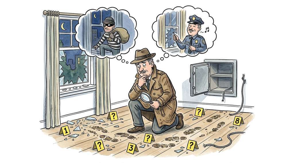
Think of abduction as a detective arriving at a crime scene. The detective sees a broken window, muddy footprints leading to an empty safe, and an alarm that was disabled. No single piece of evidence dictates the conclusion, but the detective assembles an explanation (a burglar entered through the window, walked to the safe, and cracked it after cutting the alarm) because that story, if true, would make all the evidence expected. A different detective might propose a different story (an inside job staged to look like a break-in). Abduction is the act of constructing these candidate stories, not proving which one is correct. The "selection criteria" (parsimony, testability, consistency) are the investigative follow-up: dusting for prints, checking alibis, reviewing security footage. In science, the candidate stories are hypotheses, and the follow-up is experimentation.

Computationally, abduction can be framed as an optimization problem: find the hypothesis \(H^*\) that maximizes some combination of explanatory power and simplicity. One simplified scoring function (not a formal posterior, but a useful heuristic) is:

This Bayesian formulation connects abduction to Chapter 32: Bayesian Discovery and Uncertainty, which develops the full machinery of Bayesian model comparison. The likelihood \(P(O \mid H)\) measures explanatory power (how well does the hypothesis predict the observation?), the prior \(P(H)\) encodes background plausibility, and the simplicity term implements Occam's razor.

Abduction generates candidate explanations, yet the space of possible hypotheses is vast; analogical reasoning narrows it by importing structural templates from domains where similar problems have already been solved.

4. Analogical Reasoning: Structure Mapping Across Domains

Analogical reasoning transfers knowledge from a well-understood source domain to a less-understood target domain by mapping shared structure. Rutherford modeled the atom by analogy with the solar system: electrons orbit the nucleus as planets orbit the sun. The analogy transfers relations (orbiting, gravitational/electromagnetic attraction) rather than surface features (size, color, temperature).

Dedre Gentner's Structure Mapping Theory (1983) formalizes this intuition. An analogy is good when:

1. Relational matches outnumber attribute matches (systematicity principle)
2. The mapped relations form connected, higher-order structures (not isolated pairings)
3. The mapping is one-to-one (each source element maps to exactly one target element)

The Structure Mapping Engine (SME), Gentner and Forbus's computational realization, works by: (1) finding all local matches between source and target predicates, (2) combining consistent matches into global mappings (called gmaps), and (3) scoring gmaps by structural depth. The following simplified version captures the core algorithm.

import networkx as nx
from dataclasses import dataclass, field

@dataclass
class Predicate:
    """A relational predicate: name(arg1, arg2, ...)"""
    name: str
    args: tuple[str, ...]
    is_relation: bool = True  # True for relations, False for attributes

    def __hash__(self):
        return hash((self.name, self.args))

@dataclass
class StructureMapping:
    """A mapping between source and target domain elements."""
    entity_map: dict[str, str] = field(default_factory=dict)
    predicate_matches: list[tuple[Predicate, Predicate]] = field(
        default_factory=list
    )
    score: float = 0.0

def find_analogies(
    source: list[Predicate],
    target: list[Predicate]
) -> list[StructureMapping]:
    """Simplified Structure Mapping Engine.

    Finds consistent mappings between source and target domains,
    preferring relational matches over attribute matches.
    """
    # Step 1: Find all local matches (predicates with same name)
    local_matches = []
    for s_pred in source:
        for t_pred in target:
            if (s_pred.name == t_pred.name and
                len(s_pred.args) == len(t_pred.args)):
                local_matches.append((s_pred, t_pred))

    # Step 2: Build consistent global mappings (greedy)
    mappings = []
    for s_pred, t_pred in local_matches:
        mapping = StructureMapping()
        consistent = True

        for s_arg, t_arg in zip(s_pred.args, t_pred.args):
            if s_arg in mapping.entity_map:
                if mapping.entity_map[s_arg] != t_arg:
                    consistent = False
                    break
            else:
                mapping.entity_map[s_arg] = t_arg

        if consistent:
            mapping.predicate_matches.append((s_pred, t_pred))
            # Gentner's systematicity: relations score higher
            mapping.score = sum(
                2.0 if sp.is_relation else 0.5
                for sp, _ in mapping.predicate_matches
            )
            mappings.append(mapping)

    return sorted(mappings, key=lambda m: m.score, reverse=True)

# Solar system -> Atom analogy
source_domain = [
    Predicate("revolves_around", ("planet", "sun"), is_relation=True),
    Predicate("attracts", ("sun", "planet"), is_relation=True),
    Predicate("more_massive", ("sun", "planet"), is_relation=True),
    Predicate("hot", ("sun",), is_relation=False),
    Predicate("yellow", ("sun",), is_relation=False),
]

target_domain = [
    Predicate("revolves_around", ("electron", "nucleus"), is_relation=True),
    Predicate("attracts", ("nucleus", "electron"), is_relation=True),
    Predicate("more_massive", ("nucleus", "electron"), is_relation=True),
]

analogies = find_analogies(source_domain, target_domain)
best = analogies[0]
print("Best analogy mapping:")
for src, tgt in best.entity_map.items():
    print(f"  {src} -> {tgt}")
print(f"Structural score: {best.score}")
print(f"Matched relations: {len(best.predicate_matches)}")
# Output:
# Best analogy mapping:
#   planet -> electron
#   sun -> nucleus
# Structural score: 2.0
# Matched relations: 1

Analogy suggests which relationships might hold in a new domain, but it cannot tell us which of those relationships are genuinely causal rather than merely coincidental; that distinction requires its own reasoning mode.

5. Causal Reasoning: Beyond Correlation

Causal reasoning asks not "what tends to co-occur?" but "what makes what happen?" This distinction, which we develop fully in Section 4.3, is the single most important intellectual tool for scientific discovery. An observed correlation between ice cream sales and drowning deaths does not mean ice cream causes drowning; both are caused by a common factor (summer heat).

Formally, causal reasoning requires a causal model: a directed acyclic graph (DAG; a graph whose edges have directions and that contains no loops, so causes always point forward and never circle back to themselves) whose nodes are variables and whose edges represent direct causal influence. The DAG encodes which interventions (setting a variable to a specific value, regardless of its usual causes) will affect which outcomes. This is Pearl's distinction between \(P(Y \mid X = x)\) (observing that \(X\) takes value \(x\)) and \(P(Y \mid do(X = x))\) (intervening to set \(X\) to \(x\)).

The full treatment of do-calculus appears in Section 4.3. The key distinction: statistics tells us what to expect; causal reasoning tells us what will happen if we act. For discovery AI, this is not philosophical luxury; it determines whether a system can design experiments or merely observe correlations.

Even a minimal causal model makes the observation/intervention distinction concrete. The following sketch encodes a three-variable DAG and shows how conditioning on an observation differs from intervening with do.

from dataclasses import dataclass

@dataclass
class CausalDAG:
    """A tiny causal model: edges map child -> list of parents."""
    edges: dict[str, list[str]]
    probs: dict[str, dict]  # node -> conditional probability table

    def observe(self, node: str, value: int) -> dict[str, float]:
        """P(other nodes | node = value): condition, do NOT cut edges."""
        # Simplified: return stored conditionals (full Bayes net would
        # propagate through all paths, including non-causal ones)
        return {
            "mode": "observation",
            "conditioned_on": f"{node}={value}",
            "note": "Correlations flow along ALL paths, causal or not",
        }

    def intervene(self, node: str, value: int) -> dict[str, float]:
        """P(other nodes | do(node = value)): cut incoming edges first."""
        modified_edges = {
            k: ([] if k == node else v)
            for k, v in self.edges.items()
        }
        return {
            "mode": "intervention (do-operator)",
            "set": f"do({node}={value})",
            "edges_removed": f"incoming edges to {node}",
            "note": "Only CAUSAL downstream effects remain",
            "modified_dag": modified_edges,
        }

# Ice-cream / drowning / summer-heat example
dag = CausalDAG(
    edges={
        "summer_heat": [],                   # root cause
        "ice_cream_sales": ["summer_heat"],  # heat -> ice cream
        "drowning_rate": ["summer_heat"],     # heat -> drowning
    },
    probs={}  # omitted for brevity; Section 4.3 adds full tables
)

print("Observe high ice-cream sales:")
print(dag.observe("ice_cream_sales", 1))
# Correlation with drowning_rate flows through summer_heat

print("\nIntervene to increase ice-cream sales:")
print(dag.intervene("ice_cream_sales", 1))
# do() cuts the summer_heat -> ice_cream edge;
# drowning_rate is no longer affected

6. How the Five Forms Interlock in Discovery

Systems that rely on a single reasoning mode fail in predictable ways: a purely deductive planner cannot generate novel hypotheses, a purely inductive learner cannot design the experiment that would test them, and a purely abductive engine proposes explanations it can never verify. Real scientific breakthroughs require all five modes working in concert.

The five reasoning forms are not alternatives; they are collaborators in the discovery process. Figure 4.1 illustrates how the modes feed into one another in a typical discovery cycle:

1. Induction identifies a surprising pattern in data (e.g., a new correlation)
2. Abduction generates candidate explanations for the pattern
3. Analogy transfers structural knowledge from related domains to enrich the candidates
4. Deduction derives testable predictions from each candidate hypothesis
5. Causal reasoning designs interventions that distinguish between candidates

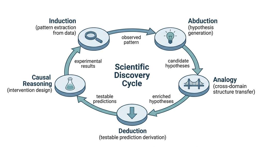
This cycle maps directly onto the scientific method covered in Chapter 2. The Discovery Workbench we build throughout this book (starting in Chapter 6) orchestrates these reasoning modes as distinct components in a pipeline architecture. In short: each reasoning mode answers a question the others cannot ask, and scientific discovery is the conversation among all five. Figure 4.1.1 illustrates the five-mode discovery reasoning cycle.

from enum import Enum, auto

class ReasoningMode(Enum):
    DEDUCTION = auto()   # Derive consequences from known rules
    INDUCTION = auto()   # Generalize from observed instances
    ABDUCTION = auto()   # Infer best explanation for observations
    ANALOGY = auto()     # Transfer structure across domains
    CAUSAL = auto()      # Distinguish correlation from mechanism

def discovery_cycle(observation: str) -> dict:
    """Orchestrate the five reasoning modes in a discovery cycle.

    This is a structural sketch; the full implementation appears
    in Section 4.4 where we build the complete pipeline.
    """
    cycle = {}

    # Step 1: What pattern did we find?
    cycle[ReasoningMode.INDUCTION] = {
        "task": "Extract pattern from observation",
        "input": observation,
        "output": "Empirical regularity or anomaly"
    }

    # Step 2: What could explain it?
    cycle[ReasoningMode.ABDUCTION] = {
        "task": "Generate candidate explanations",
        "input": "Observed pattern + background knowledge",
        "output": "Ranked list of hypotheses"
    }

    # Step 3: Do similar phenomena exist elsewhere?
    cycle[ReasoningMode.ANALOGY] = {
        "task": "Find structural parallels in other domains",
        "input": "Candidate hypotheses + domain knowledge base",
        "output": "Enriched hypotheses with transferred structure"
    }

    # Step 4: What would each hypothesis predict?
    cycle[ReasoningMode.DEDUCTION] = {
        "task": "Derive testable predictions",
        "input": "Each candidate hypothesis",
        "output": "Observable consequences per hypothesis"
    }

    # Step 5: What experiment distinguishes them?
    cycle[ReasoningMode.CAUSAL] = {
        "task": "Design discriminating interventions",
        "input": "Predictions + causal model",
        "output": "Experimental protocol"
    }

    return cycle

# Example: unexpected drug interaction observed
result = discovery_cycle(
    "Patients taking Drug A and Drug B show unexpected liver enzyme elevation"
)
for mode, step in result.items():
    print(f"{mode.name:12s} -> {step['task']}")