4.3 Causal Reasoning and the Do-Calculus

"Correlation told me everything I wanted to hear. Causation told me everything I needed to know. I still preferred correlation. It was nicer."

A Causal Graph With Too Many Confounders

1. The Ladder of Causation

A hospital notices that patients who receive a new drug recover faster, so it recommends the drug to everyone. Mortality rises instead of falling. Wealthier patients had been choosing the drug and recovering for reasons unrelated to it. Why did a reasonable inference from real data produce the opposite of the truth? No amount of additional data can bridge the gap between observing an association and intervening on a cause. Pearl's "ladder of causation" organizes this distinction into three levels, each strictly more powerful than the one below:

1. Association (seeing): \(P(Y \mid X)\). "Patients who take the drug have lower mortality." This is what observational data gives us. No causal claim is warranted.
2. Intervention (doing): \(P(Y \mid do(X))\). "If we administer the drug, mortality will decrease." This is what a randomized controlled trial answers. It requires either experimental data or the do-calculus.
3. Counterfactual (imagining): \(P(Y_x \mid X = x', Y = y')\). "Would this specific patient have survived if we had given the drug, given that we did not and the patient died?" This is the most powerful level, requiring the full structural causal model.

The critical insight: you cannot climb the ladder using data alone. No amount of observational data (level 1) can answer an interventional question (level 2) without additional causal assumptions. This is not a limitation of sample size or statistical power; it is a mathematical impossibility. The do-calculus provides the minimum set of assumptions (encoded as a causal DAG) needed to bridge the gap. In short: Data alone tells you what happened; only causal assumptions can tell you what would happen if you intervened.

Mental Model

Think of the three rungs as three ways of reasoning about an ice cream shop on a hot day. Association is reading the sales log: "On days when we sold a lot of ice cream, the local pool was also crowded." You see the correlation but cannot tell whether ice cream drives pool attendance. Intervention is running an experiment: you shut down the shop for a week and observe that pool attendance stays the same, proving ice cream sales do not cause pool visits (the hidden cause is temperature). Counterfactual is the most specific: "Given that last Tuesday was 35 degrees and we sold 400 cones, would we have sold only 100 if the temperature had been 18 degrees?" Each rung demands strictly more knowledge: the sales log alone (no matter how large) cannot tell you what closing the shop would do, and the closure experiment cannot tell you what would have happened on a specific past day under different weather. The ladder is not about better data; it is about a qualitatively different kind of question, each requiring its own kind of causal assumption.

2. Causal DAGs and the Do-Operator

In 2020, a widely cited observational study reported that hydroxychloroquine appeared to reduce COVID-19 mortality, a finding that evaporated once randomized trials controlled for the confounders the original analysis had ignored. The tool that explains why the two analyses diverged, and that predicts such divergences before lives are at stake, is the causal DAG paired with the do-operator.

A causal DAG (directed acyclic graph) represents the qualitative causal structure of a system. Each node is a variable; each directed edge \(X \rightarrow Y\) means "\(X\) is a direct cause of \(Y\)." The graph encodes two kinds of information: what causes what, and (equally important) what does not cause what (missing edges).

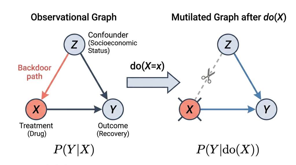
The do-operator, written $do(X = x)$, represents an intervention that sets variable \(X\) to value \(x\) regardless of its natural causes. Graphically, $do(X = x)$ means deleting all incoming edges to \(X\) (severing it from its parents) and fixing \(X = x\). The resulting mutilated graph captures the post-intervention causal structure. Figure 4.3.1 illustrates do-operator graph surgery and the mutilated graph.

Why the Do-Operator Matters

The do-operator bridges observational statistics and experimental science. It translates "what would happen if we force \(X\) to take value \(x\)?" into a precise mathematical object, \(P(Y \mid do(X = x))\), comparable with the purely observational \(P(Y \mid X = x)\). These two quantities can diverge wildly whenever confounders exist. Confusing them is the root cause of most spurious causal claims from observational data. The mechanism is graph surgery: deleting every incoming edge to \(X\) simulates an idealized randomized experiment. \(X\) is assigned externally, breaking all associations with its natural causes. The do-operator (and the do-calculus that manipulates it) applies when causal conclusions must come from non-experimental data. When a true randomized experiment is feasible and ethical, it provides \(P(Y \mid do(X))\) directly without requiring DAG assumptions.

Consider the classic confounding example. Let \(Z\) be socioeconomic status, \(X\) be whether a patient receives a drug, and \(Y\) be recovery. Figure 4.3 shows the original DAG alongside the mutilated graph produced by \(do(X)\):

In this graph, \(Z\) confounds the relationship between \(X\) and \(Y\). Wealthier patients (\(Z\) high) both receive the drug more often (\(Z \rightarrow X\)) and recover more often for other reasons (\(Z \rightarrow Y\)). The observational quantity \(P(Y \mid X)\) mixes the drug's true effect with the confounding effect of wealth. The interventional quantity \(P(Y \mid do(X))\) isolates the drug's true effect by severing the \(Z \rightarrow X\) edge.

import networkx as nx
import matplotlib
matplotlib.use("Agg")
import matplotlib.pyplot as plt

def build_causal_dag(edges: list[tuple[str, str]]) -> nx.DiGraph:
    """Build a causal DAG from a list of directed edges."""
    G = nx.DiGraph()
    G.add_edges_from(edges)
    assert nx.is_directed_acyclic_graph(G), "Graph has cycles!"
    return G

def mutilate(G: nx.DiGraph, intervention_node: str) -> nx.DiGraph:
    """Apply do-operator: remove all incoming edges to the intervention node.

    This produces the 'mutilated graph' G_X that represents
    the causal structure after the intervention do(X=x).
    """
    G_mutilated = G.copy()
    parents = list(G_mutilated.predecessors(intervention_node))
    for parent in parents:
        G_mutilated.remove_edge(parent, intervention_node)
    return G_mutilated

# Confounding example: Z -> X, Z -> Y, X -> Y
dag = build_causal_dag([("Z", "X"), ("Z", "Y"), ("X", "Y")])

print("Original DAG edges:", list(dag.edges()))
# Output: [('Z', 'X'), ('Z', 'Y'), ('X', 'Y')]

# Apply do(X): sever Z -> X
dag_do_x = mutilate(dag, "X")
print("After do(X) edges:", list(dag_do_x.edges()))
# Output: [('Z', 'Y'), ('X', 'Y')]

# In the mutilated graph, Z no longer confounds X -> Y
# because Z has no path to X

3. The Backdoor Criterion

Graph mutilation tells us what the post-intervention world looks like, but we still need a practical test for when the interventional distribution can be computed from observational data alone; the backdoor criterion provides exactly that test.

The backdoor criterion (Pearl, 1993) provides a sufficient condition for identifying causal effects from observational data. A set of variables \(\mathbf{Z}\) satisfies the backdoor criterion relative to \((X, Y)\) if:

1. No node in \(\mathbf{Z}\) is a descendant of \(X\)
2. \(\mathbf{Z}\) blocks every path between \(X\) and \(Y\) that contains an arrow into \(X\) (a "backdoor path," where information flows from \(Y\) to \(X\) through a common cause rather than along the causal direction)

When a valid backdoor set \(\mathbf{Z}\) exists, the causal effect is identifiable via the adjustment formula:

This is the mathematical justification for "controlling for confounders" in statistical analysis. The formula says: to compute the effect of intervening on \(X\), condition on \(X\) and the confounders \(\mathbf{Z}\), then average over the natural distribution of \(\mathbf{Z}\).

def find_backdoor_paths(
    G: nx.DiGraph,
    treatment: str,
    outcome: str
) -> list[list[str]]:
    """Find all backdoor paths from treatment to outcome.

    A backdoor path starts with an arrow INTO treatment
    (i.e., goes through a parent of treatment).
    """
    backdoor_paths = []
    # Convert to undirected for path finding, but track direction
    G_undirected = G.to_undirected()

    for path in nx.all_simple_paths(G_undirected, treatment, outcome):
        if len(path) < 2:
            continue
        # A backdoor path has an arrow INTO treatment at the first step
        # i.e., path[1] -> treatment exists in original DAG
        if G.has_edge(path[1], treatment):
            backdoor_paths.append(path)

    return backdoor_paths

def satisfies_backdoor(
    G: nx.DiGraph,
    treatment: str,
    outcome: str,
    adjustment_set: set[str]
) -> bool:
    """Check if adjustment_set satisfies the backdoor criterion.

    Conditions:
    1. No node in adjustment_set is a descendant of treatment
    2. adjustment_set blocks all backdoor paths
    """
    # Condition 1: no descendants of treatment
    descendants = nx.descendants(G, treatment)
    if adjustment_set & descendants:
        return False

    # Condition 2: blocks all backdoor paths
    backdoor_paths = find_backdoor_paths(G, treatment, outcome)
    for path in backdoor_paths:
        # A path is blocked if any node in it (except endpoints)
        # is in the adjustment set
        interior = set(path[1:-1])
        if not (interior & adjustment_set):
            return False  # This path is not blocked

    return True

# Extended example: Drug trial with confounder and mediator
# Z (socioeconomic) -> X (drug), Z -> Y (recovery)
# X -> M (biomarker) -> Y
dag = build_causal_dag([
    ("Z", "X"), ("Z", "Y"), ("X", "M"), ("M", "Y")
])

# Test various adjustment sets
for adj_set in [{"Z"}, {"M"}, {"Z", "M"}, set()]:
    valid = satisfies_backdoor(dag, "X", "Y", adj_set)
    print(f"  Adjust for {adj_set or '{}'}: {'VALID' if valid else 'INVALID'}")
# Output:
#   Adjust for {'Z'}: VALID
#   Adjust for {'M'}: INVALID (M is a descendant of X)
#   Adjust for {'Z', 'M'}: INVALID (M is a descendant of X)
#   Adjust for {}: INVALID (backdoor Z->X not blocked)

4. The Frontdoor Criterion

What if no valid backdoor adjustment set exists? The frontdoor criterion handles a specific but important case: when the treatment affects the outcome only through a mediator \(M\), and the confounder \(U\) does not directly affect \(M\). The strategy is to decompose the overall causal effect into two sub-effects (treatment on mediator, mediator on outcome), each of which can be identified individually, and then compose them.

Here \(U\) is unobserved (no data available), so we cannot adjust for it. Yet the frontdoor criterion lets us identify the causal effect of \(X\) on \(Y\) through \(M\):

The intuition: first identify how \(X\) affects \(M\) (unconfounded because \(U\) does not affect \(M\) directly), then identify how \(M\) affects \(Y\) (using \(X\) as a backdoor adjustment for \(M \rightarrow Y\)), and compose the two effects.

5. The Three Rules of Do-Calculus

The backdoor and frontdoor criteria are special cases of Pearl's do-calculus, a complete system for causal identification: if a causal effect can be identified from a DAG, these three rules (plus standard probability) suffice to derive the formula. In particular, both the backdoor adjustment formula (Section 3) and the frontdoor formula (Section 4) can be derived by applying these rules in sequence to their respective graphs. (Three rules. That is the entire calculus. Every identifiable causal effect in every possible graph yields to some sequence of just these three transformations.)

Let \(G\) be a causal DAG, \(X\), \(Y\), \(Z\), \(W\) be disjoint sets of variables, and let \(G_{\overline{X}}\) denote the graph with incoming edges to \(X\) removed, \(G_{\underline{X}}\) denote the graph with outgoing edges from \(X\) removed.

Rule 1 (Insertion/deletion of observations):

We can add or remove an observation \(Z\) if \(Y\) and \(Z\) are d-separated (conditionally independent given the graph structure; informally, every path between them is "blocked" by either a non-collider in the conditioning set or a collider outside it) in the manipulated graph.

Rule 2 (Action/observation exchange):

We can replace \(do(Z)\) with observation \(Z\) (or vice versa) if \(Y\) and \(Z\) are d-separated in the graph where incoming edges to \(X\) and outgoing edges from \(Z\) are removed.

Rule 3 (Insertion/deletion of actions):

where \(Z(S)\) is the set of nodes in \(Z\) that are not ancestors of any node in \(W\) in \(G_{\overline{X}}\). We can remove the action \(do(Z)\) entirely if \(Y\) and \(Z\) are d-separated in the appropriately manipulated graph.

def d_separated(
    G: nx.DiGraph,
    X: set[str],
    Y: set[str],
    Z: set[str]
) -> bool:
    """Test d-separation in a DAG: X _||_ Y | Z.

    Uses the Bayes-Ball algorithm (Shachter, 1998), a message-passing
    procedure that traces which nodes are reachable from X given the
    conditioning set Z, respecting the direction of edges and collider
    blocking rules.
    Returns True if X and Y are d-separated given Z.
    """
    # Build ancestor set of Z for collider unblocking
    z_ancestors = set()
    for z in Z:
        z_ancestors |= nx.ancestors(G, z)
    z_ancestors |= Z

    # BFS from X nodes, tracking direction of traversal
    # States: (node, direction) where direction is "up" or "down"
    visited = set()
    queue = []

    for x in X:
        queue.append((x, "up"))
        queue.append((x, "down"))

    reachable = set()

    while queue:
        node, direction = queue.pop(0)
        if (node, direction) in visited:
            continue
        visited.add((node, direction))

        if node in Y:
            reachable.add(node)

        # If arriving from a child (going "up")
        if direction == "up" and node not in Z:
            # Continue to parents (up)
            for parent in G.predecessors(node):
                queue.append((parent, "up"))
            # Continue to children (down)
            for child in G.successors(node):
                queue.append((child, "down"))

        # If arriving from a parent (going "down")
        elif direction == "down":
            # If not in Z, pass through to children
            if node not in Z:
                for child in G.successors(node):
                    queue.append((child, "down"))
            # If in Z or ancestor of Z, collider is unblocked: go up
            if node in z_ancestors:
                for parent in G.predecessors(node):
                    queue.append((parent, "up"))

    return len(reachable) == 0

def apply_do_calculus_rule2(
    G: nx.DiGraph,
    Y: str,
    X: str,
    Z: str,
    W: set[str]
) -> bool:
    """Check if Rule 2 applies: can we replace do(Z) with observation Z?

    Requires: Y _||_ Z | (X, W) in G with incoming edges to X removed
    and outgoing edges from Z removed.
    """
    # Build G_{overline{X}, underline{Z}}
    G_modified = G.copy()

    # Remove incoming edges to X (overline)
    for parent in list(G_modified.predecessors(X)):
        G_modified.remove_edge(parent, X)

    # Remove outgoing edges from Z (underline)
    for child in list(G_modified.successors(Z)):
        G_modified.remove_edge(Z, child)

    # Test d-separation
    conditioning = {X} | W
    return d_separated(G_modified, {Z}, {Y}, conditioning)

# Test on the frontdoor graph: U -> X, U -> Y, X -> M -> Y
frontdoor_dag = build_causal_dag([
    ("U", "X"), ("U", "Y"), ("X", "M"), ("M", "Y")
])

# Can we replace do(X) with observation X when estimating
# the effect on M? (Step 1 of frontdoor)
can_exchange = apply_do_calculus_rule2(
    frontdoor_dag, Y="M", X="X", Z="X", W=set()
)
print(f"Rule 2 applicable (M, do(X) -> obs X): {can_exchange}")
# Output: True (because U does not affect M except through X)

6. Counterfactual Reasoning

The do-calculus settles what we can learn about populations under interventions, but science often demands a more personal question: what would have happened to this particular patient, experiment, or observation under different circumstances?

The highest rung of Pearl's ladder is counterfactual reasoning: "What would have happened if things had been different?" Counterfactuals require a full structural causal model (SCM), not just a DAG. An SCM specifies the functional form of each variable:

where \(\text{pa}(X_i)\) are the parents of \(X_i\) in the DAG and \(U_i\) is an exogenous noise variable (a factor determined entirely outside the model, representing unmodeled influences on \(X_i\)). Given an SCM and observed evidence, counterfactual reasoning proceeds in three steps:

1. Abduction: Use the observed evidence to infer the values of exogenous variables \(U_i\)
2. Action: Modify the SCM according to the hypothetical intervention
3. Prediction: Compute the outcome in the modified model with the inferred \(U_i\) values

import numpy as np

class StructuralCausalModel:
    """A simple linear structural causal model for counterfactual reasoning."""

    def __init__(self):
        self.equations = {}   # node -> (coefficients_dict, noise_std)
        self.noise_values = {}  # Realized noise (set during abduction)

    def add_equation(
        self,
        variable: str,
        parents: dict[str, float],
        noise_std: float = 1.0
    ):
        """Add structural equation: variable = sum(coeff * parent) + noise."""
        self.equations[variable] = (parents, noise_std)

    def sample(self, n: int = 1, seed: int = 42) -> dict[str, np.ndarray]:
        """Generate observational samples from the SCM."""
        rng = np.random.default_rng(seed)
        data = {}

        for var in self._topological_order():
            parents, noise_std = self.equations[var]
            value = rng.normal(0, noise_std, size=n)
            for parent, coeff in parents.items():
                value = value + coeff * data[parent]
            data[var] = value

        return data

    def counterfactual(
        self,
        observed: dict[str, float],
        intervention: dict[str, float],
        query: str
    ) -> float:
        """Compute a counterfactual: P(query | observed, do(intervention)).

        Step 1 (Abduction): Infer noise from observations
        Step 2 (Action): Apply intervention
        Step 3 (Prediction): Compute query under modified model
        """
        # Step 1: Abduction - infer noise values from observations
        noise = {}
        for var in self._topological_order():
            parents, _ = self.equations[var]
            if var in observed:
                # noise = observed - sum(coeff * parent_value)
                parent_contribution = sum(
                    coeff * observed.get(p, 0.0) for p, coeff in parents.items()
                )
                noise[var] = observed[var] - parent_contribution
            else:
                noise[var] = 0.0  # Use expected noise for unobserved

        # Step 2 & 3: Action + Prediction with inferred noise
        values = {}
        for var in self._topological_order():
            if var in intervention:
                values[var] = intervention[var]  # Intervened: fixed value
            else:
                parents, _ = self.equations[var]
                value = noise[var]
                for parent, coeff in parents.items():
                    value += coeff * values[parent]
                values[var] = value

        return values[query]

    def _topological_order(self) -> list[str]:
        """Return variables in topological order."""
        G = nx.DiGraph()
        for var, (parents, _) in self.equations.items():
            for parent in parents:
                G.add_edge(parent, var)
            if not parents:
                G.add_node(var)
        return list(nx.topological_sort(G))

# Example: Drug dosage -> Biomarker -> Recovery
# With confounder Age affecting both Dosage and Recovery
scm = StructuralCausalModel()
scm.add_equation("Age", {}, noise_std=10.0)         # Exogenous
scm.add_equation("Dosage", {"Age": -0.1}, noise_std=2.0)  # Older -> less drug
scm.add_equation("Biomarker", {"Dosage": 0.5}, noise_std=1.0)
scm.add_equation("Recovery", {"Biomarker": 0.8, "Age": -0.05}, noise_std=1.0)

# Observed patient: Age=60, Dosage=2, Biomarker=1.5, Recovery=0.7
observed = {"Age": 60.0, "Dosage": 2.0, "Biomarker": 1.5, "Recovery": 0.7}

# Counterfactual: what if we had given Dosage=10?
cf_recovery = scm.counterfactual(
    observed=observed,
    intervention={"Dosage": 10.0},
    query="Recovery"
)
print(f"Observed recovery:       {observed['Recovery']:.2f}")
print(f"Counterfactual recovery: {cf_recovery:.2f}")
print(f"Estimated treatment effect: {cf_recovery - observed['Recovery']:.2f}")
# Output:
# Observed recovery:       0.70
# Counterfactual recovery:  3.90
# Estimated treatment effect: 3.20

7. Causal Identification in Practice

For discovery AI practitioners, the operational question is: "Given my causal DAG and available data, can I identify the causal effect I care about, and if so, what formula should I use?" The following algorithm automates this process for simple cases:

from dataclasses import dataclass
from enum import Enum, auto

class IdentificationResult(Enum):
    BACKDOOR = auto()
    FRONTDOOR = auto()
    NOT_IDENTIFIED = auto()

@dataclass
class CausalQuery:
    treatment: str
    outcome: str
    dag: nx.DiGraph
    observed: set[str]  # Variables we can measure

def identify_effect(query: CausalQuery) -> tuple[IdentificationResult, str]:
    """Attempt to identify a causal effect using standard criteria.

    Tries backdoor first (simpler), then frontdoor.
    Returns the identification method and adjustment formula.
    """
    G = query.dag
    X, Y = query.treatment, query.outcome

    # Try backdoor: find a valid adjustment set among observed variables
    candidates = query.observed - {X, Y}
    descendants_X = nx.descendants(G, X)

    # Try subsets of candidates (smallest first for parsimony)
    from itertools import combinations
    for size in range(len(candidates) + 1):
        for subset in combinations(candidates, size):
            adj_set = set(subset)
            if adj_set & descendants_X:
                continue  # Violates condition 1
            if satisfies_backdoor(G, X, Y, adj_set):
                formula = (
                    f"P({Y}|do({X})) = "
                    f"Sum_({','.join(adj_set) or 'none'}) "
                    f"P({Y}|{X},{','.join(adj_set)}) * "
                    f"P({','.join(adj_set)})"
                )
                return IdentificationResult.BACKDOOR, formula

    # Try frontdoor: find mediator M where X -> M -> Y
    for M in query.observed - {X, Y}:
        if G.has_edge(X, M) and nx.has_path(G, M, Y):
            # Check: no unblocked backdoor path from X to M
            if satisfies_backdoor(G, X, M, set()):
                formula = (
                    f"P({Y}|do({X})) = "
                    f"Sum_{M} P({M}|{X}) * "
                    f"Sum_{X}' P({Y}|{X}',{M}) * P({X}')"
                )
                return IdentificationResult.FRONTDOOR, formula

    return IdentificationResult.NOT_IDENTIFIED, "Effect not identifiable"

# Test 1: Simple confounding (backdoor works)
simple_dag = build_causal_dag([("Z", "X"), ("Z", "Y"), ("X", "Y")])
q1 = CausalQuery("X", "Y", simple_dag, {"X", "Y", "Z"})
result, formula = identify_effect(q1)
print(f"Simple confounding: {result.name}")
print(f"  Formula: {formula}")

# Test 2: Unobserved confounding with mediator (frontdoor works)
frontdoor_dag = build_causal_dag([
    ("U", "X"), ("U", "Y"), ("X", "M"), ("M", "Y")
])
q2 = CausalQuery("X", "Y", frontdoor_dag, {"X", "Y", "M"})  # U unobserved
result2, formula2 = identify_effect(q2)
print(f"\nUnobserved confounding: {result2.name}")
print(f"  Formula: {formula2}")
# Output:
# Simple confounding: BACKDOOR
#   Formula: P(Y|do(X)) = Sum_(Z) P(Y|X,Z) * P(Z)
# Unobserved confounding: FRONTDOOR
#   Formula: P(Y|do(X)) = Sum_M P(M|X) * Sum_X' P(Y|X',M) * P(X')