31.1 Structural Causal Models

1. The Four-Tuple Formalism

When a pharmaceutical company asks whether its new drug truly lowers blood pressure or merely correlates with patients who were already healthier, the answer depends on four mathematical objects that, together, separate genuine causes from statistical mirages. A structural causal model is a four-tuple \(\mathcal{M} = (V, U, F, P_U)\), and each component captures a distinct aspect of that causal story:

The four-tuple formalism provides the minimal mathematical specification needed to answer "what if?" questions about a system. \(V\) names what you measure. \(U\) captures everything you do not measure. \(F\) encodes the directional mechanisms by which causes produce effects. \(P_U\) injects the randomness that makes outcomes probabilistic rather than deterministic. Without all four components, you cannot distinguish genuine causal effects from confounded associations. The formalism forces you to commit to a specific generative story before computing any effects. The mechanism is straightforward: given a draw from \(P_U\), each structural equation in \(F\) fires in topological order (where every parent node is evaluated before its children) along the DAG, deterministically producing every endogenous variable from its direct causes and its noise term. Use an SCM when your scientific question involves interventions or counterfactuals; use a standard probabilistic graphical model (such as a Bayesian network) when prediction under passive observation is sufficient and causal commitments are unnecessary.

• \(V = \{V_1, \ldots, V_n\}\): the endogenous variables, the quantities we observe and care about. In a clinical trial, these might be treatment assignment, patient age, blood pressure, and mortality.
• \(U = \{U_1, \ldots, U_m\}\): the exogenous variables, background factors determined outside the model. These represent everything we do not (or cannot) measure: genetic predispositions, environmental exposures, measurement noise.
• \(F = \{f_1, \ldots, f_n\}\): the structural equations, one per endogenous variable. Each \(f_i\) is a deterministic function \(V_i = f_i(\text{pa}(V_i), U_i)\) specifying how \(V_i\) is generated from its direct causes \(\text{pa}(V_i) \subseteq V \setminus \{V_i\}\) and its exogenous noise \(U_i\).
• \(P_U\): a joint probability distribution over the exogenous variables. All randomness in the model flows through \(P_U\); given a realization of \(U\), every endogenous variable is determined.

The structural equations are not regression equations, and this distinction is crucial. A regression \(Y = \beta X + \epsilon\) is a statistical statement about association: it describes how to predict \(Y\) from \(X\) in the observed data. A structural equation \(Y := f(X, U_Y)\) is a causal statement about mechanism: it asserts that the value of \(Y\) is generated by applying \(f\) to the values of its causes \(X\) and noise \(U_Y\). The asymmetric notation $:=$ (or \(\leftarrow\)) emphasizes that the left-hand variable is produced by the right-hand side, not merely correlated with it. In short: an SCM is a bet on the wiring diagram of reality; get the arrows right, and the math tells you what every intervention will do before you touch a single variable.

Let us build a concrete SCM for a scientific scenario. Suppose we study the effect of a new fertilizer (\(T\)) on crop yield (\(Y\)), where soil quality (\(S\)) affects both the farmer's decision to use the fertilizer and the yield itself:

Here \(S\) is a confounder: it causes both treatment (\(T\)) and outcome (\(Y\)). If we simply regress \(Y\) on \(T\), the coefficient will absorb part of the effect of \(S\), inflating the apparent benefit of the fertilizer. The SCM makes this confounding structure explicit through the DAG implied by the structural equations, as shown in Figure 31.1.

2. Directed Acyclic Graphs and d-Separation

Every SCM \(\mathcal{M}\) induces a DAG \(\mathcal{G}\) where each node represents an endogenous variable and each directed edge \(V_i \to V_j\) indicates that \(V_i\) appears as an argument in the structural equation for \(V_j\). The DAG encodes the qualitative causal structure: which variables directly cause which others. In our fertilizer example, the DAG has edges \(S \to T\), \(S \to Y\), and \(T \to Y\).

The graph's power comes from d-separation, a graphical criterion that reads conditional independence relations directly from the DAG structure. Two variables \(X\) and \(Y\) are d-separated by a set \(Z\) (written \(X \perp\!\!\!\perp_{\mathcal{G}} Y \mid Z\)) if every path between \(X\) and \(Y\) is "blocked" by \(Z\). A path is blocked by \(Z\) if it contains:

• A chain \(A \to B \to C\) where \(B \in Z\) (conditioning on the mediator blocks the information flow).
• A fork \(A \leftarrow B \to C\) where \(B \in Z\) (conditioning on the common cause removes the spurious association).
• A collider \(A \to B \leftarrow C\) where \(B \notin Z\) and no descendant of \(B\) is in \(Z\) (the path is already blocked unless we condition on the collider or its descendant).

The causal Markov condition (the assumption that each variable is independent of its non-descendants given its direct causes) connects the graph to the probability distribution. If the DAG \(\mathcal{G}\) is the causal graph for the data-generating process, every d-separation in \(\mathcal{G}\) implies a conditional independence in the observed distribution \(P(V)\). The converse, the faithfulness assumption (the assumption that the only conditional independencies in \(P(V)\) are those implied by d-separation in the graph, ruling out coincidental cancellations among parameters), asserts that d-separation accounts for all conditional independencies in \(P(V)\). Together, these two assumptions let you read testable predictions from the graph and, running in reverse, learn graph structure from conditional independence tests (as covered in Section 31.2).

import networkx as nx
import matplotlib.pyplot as plt

# Build the fertilizer DAG
dag = nx.DiGraph()
dag.add_edges_from([
    ("SoilQuality", "Treatment"),
    ("SoilQuality", "Yield"),
    ("Treatment", "Yield"),
])

# Check d-separation: is Treatment independent of Yield given SoilQuality?
# In this DAG, conditioning on SoilQuality blocks the backdoor path
# but also blocks the direct causal path T -> Y (it doesn't, actually,
# because SoilQuality is not on the direct path T -> Y).
# Let's verify with networkx's d-separation check:
is_dsep = nx.d_separated(dag, {"Treatment"}, {"Yield"}, {"SoilQuality"})
print(f"T _||_ Y | S? {is_dsep}")  # False: direct path T -> Y remains open

# What about T _||_ Y | {} (unconditionally)?
is_dsep_empty = nx.d_separated(dag, {"Treatment"}, {"Yield"}, set())
print(f"T _||_ Y | {{}}? {is_dsep_empty}")  # False: both paths open

3. The do-Operator and Interventions

Knowing which variables are d-separated in a graph tells us what the data alone can and cannot reveal, but the real payoff of encoding causal structure is the ability to predict what happens when we actively change a variable rather than passively observe it.

The central innovation of Pearl's framework is the do-operator, which formalizes the difference between observing that \(X = x\) and intervening to set \(X = x\). The interventional distribution \(P(Y \mid \text{do}(X = x))\) describes the distribution of \(Y\) that would result from physically forcing \(X\) to equal \(x\), overriding whatever natural process normally generates \(X\).

Mechanically, the do-operator works by graph surgery (we walk through a concrete numeric example in the step-through box below): to compute \(P(Y \mid \text{do}(X = x))\), we take the original SCM, delete all edges pointing into \(X\) (removing the influence of \(X\)'s natural causes), set \(X = x\), and propagate forward through the remaining structural equations. This yields the truncated factorization (the joint distribution rewritten with the intervened variable's factor removed, so that \(X\) no longer depends on its original causes): Figure 31.1.1 illustrates graph surgery and the do-operator.

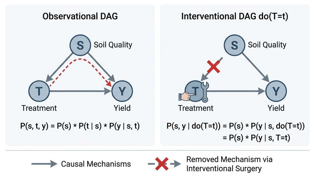
Compare this with the ordinary conditional distribution \(P(Y \mid X = x)\), which conditions on observing \(X = x\) without changing the data-generating process. When \(X\) has causes that also affect \(Y\) (confounders), \(P(Y \mid X = x)\) and \(P(Y \mid \text{do}(X = x))\) diverge. The do-operator captures the causal effect; the conditional captures the associational relationship.

import numpy as np
import pandas as pd

np.random.seed(42)
n = 10_000

# Generate data from the fertilizer SCM
U_S = np.random.normal(0, 1, n)
U_T = np.random.normal(0, 1, n)
U_Y = np.random.normal(0, 1, n)

S = U_S  # Soil quality
T = (0.5 * S + U_T > 0).astype(float)  # Treatment (binary)
Y = 2 * T + 0.8 * S + U_Y  # Yield

data = pd.DataFrame({"S": S, "T": T, "Y": Y})

# Naive (confounded) estimate: E[Y|T=1] - E[Y|T=0]
naive_ate = data[data.T == 1]["Y"].mean() - data[data.T == 0]["Y"].mean()
print(f"Naive ATE (confounded): {naive_ate:.3f}")  # ~2.4, biased upward

# True ATE from the structural equation: coefficient of T in Y := 2T + 0.8S + U_Y
print(f"True ATE: 2.000")

# Adjustment formula: E[Y|do(T=t)] = sum_s E[Y|T=t, S=s] P(S=s)
# With continuous S, we use regression adjustment
from sklearn.linear_model import LinearRegression

model = LinearRegression()
model.fit(data[["T", "S"]], data["Y"])
print(f"Adjusted ATE (regression): {model.coef_[0]:.3f}")  # ~2.0, correct

4. The Backdoor Criterion

The adjustment formula in Listing 31.2 worked because soil quality \(S\) satisfied the backdoor criterion. A set of variables \(Z\) satisfies the backdoor criterion relative to an ordered pair \((X, Y)\) in a DAG \(\mathcal{G}\) if:

1. No node in \(Z\) is a descendant of \(X\).
2. \(Z\) blocks every path between \(X\) and \(Y\) that contains an arrow into \(X\) (a "backdoor path").

When a set \(Z\) satisfies the backdoor criterion, the causal effect of \(X\) on \(Y\) is identified by the backdoor adjustment formula:

This formula converts the interventional query (left side) into a purely observational computation (right side): condition on \(X\) and \(Z\), then marginalize over \(Z\). The key insight is that conditioning on a valid adjustment set \(Z\) blocks all non-causal (backdoor) paths between \(X\) and \(Y\) while leaving all causal (directed) paths open.

5. The Front-Door Criterion

The backdoor criterion requires that we can measure and adjust for all confounders. When some confounders are unmeasured, the backdoor criterion fails. The front-door criterion provides an alternative identification strategy when there is a fully observed mediator \(M\) on the causal path from \(X\) to \(Y\).

A set of variables \(M\) satisfies the front-door criterion relative to \((X, Y)\) if:

1. \(M\) intercepts all directed paths from \(X\) to \(Y\).
2. There is no unblocked backdoor path from \(X\) to \(M\).
3. All backdoor paths from \(M\) to \(Y\) are blocked by \(X\).

When the front-door criterion holds, the causal effect is identified by:

The classic example is the smoking-cancer-tar deposits triangle. Suppose an unmeasured genetic factor \(U\) affects both smoking behavior and lung cancer risk. We cannot use the backdoor criterion because \(U\) is unobserved. But if all of smoking's effect on cancer goes through tar deposits in the lungs, and if there is no direct path from genetics to tar deposits except through smoking, then tar deposits satisfy the front-door criterion, and we can identify the causal effect of smoking on cancer.

import dowhy
from dowhy import CausalModel

# Simulate front-door scenario
np.random.seed(42)
n = 5_000

U = np.random.normal(0, 1, n)  # Unmeasured confounder
X = 0.6 * U + np.random.normal(0, 1, n)  # Treatment (affected by confounder)
M = 0.7 * X + np.random.normal(0, 0.5, n)  # Mediator (only caused by X)
Y = 0.9 * M + 0.5 * U + np.random.normal(0, 0.5, n)  # Outcome (M + confounder)

df = pd.DataFrame({"X": X, "M": M, "Y": Y})

# True effect of do(X) on Y through M: 0.7 * 0.9 = 0.63
print(f"True causal effect (X -> M -> Y): {0.7 * 0.9:.2f}")

# DoWhy with front-door specification
model = CausalModel(
    data=df,
    treatment="X",
    outcome="Y",
    graph="""digraph {
        U [unobserved];
        U -> X; U -> Y;
        X -> M; M -> Y;
    }""",
)

# Identify the estimand (should find front-door)
identified = model.identify_effect(proceed_when_unidentifiable=True)
print(identified)

# Estimate using the front-door formula
estimate = model.estimate_effect(
    identified,
    method_name="frontdoor.two_stage_regression",
)
print(f"Front-door estimate: {estimate.value:.3f}")

Real-World Application: Uber's Surge Pricing

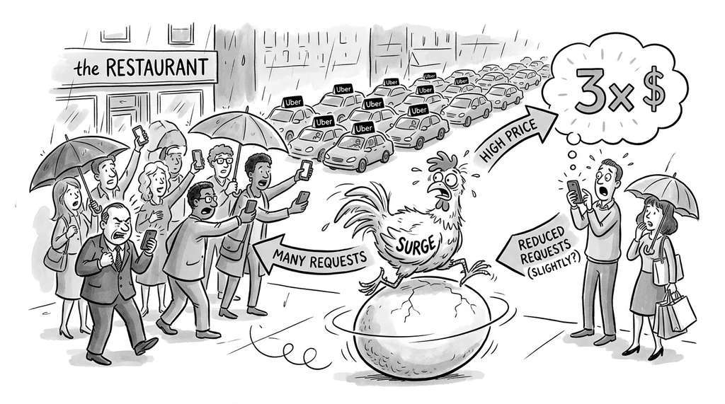
Uber's marketplace team has reportedly used structural causal models to estimate how surge pricing affects rider demand. The challenge is that surge prices are triggered by high demand, creating a feedback loop (confounder) between price and ride requests. By encoding the time-of-day, weather, and local event schedule as exogenous causes of both surge activation and rider intent, the team applies backdoor adjustment to isolate the causal elasticity of price on completed rides. This SCM-based approach replaced earlier A/B tests that were operationally expensive and ethically fraught (randomly charging different prices in the same area), enabling continuous causal monitoring from observational logs alone.

6. Beyond Backdoor and Front-Door: The do-Calculus

The backdoor and front-door criteria each handle a specific graph topology, but many real-world causal graphs do not fit neatly into either pattern, motivating a more general identification machinery.

The backdoor and front-door criteria are special cases of Pearl's do-calculus, a complete set of three inference rules that can determine whether any causal query is identifiable from any combination of observational and interventional data. The three rules govern when we can:

1. Rule 1 (Insertion/deletion of observations): Add or remove a conditioning variable when it is d-separated from \(Y\) in a modified graph.
2. Rule 2 (Action/observation exchange): Replace \(\text{do}(X = x)\) with observation \(X = x\) when \(X\) is d-separated from \(Y\) in the graph with incoming edges to \(X\) removed.
3. Rule 3 (Insertion/deletion of actions): Remove \(\text{do}(X = x)\) when \(X\) has no causal effect on \(Y\) in a modified graph.

The do-calculus is provably complete (Huang and Valtorta, 2006; Shpitser and Pearl, 2006): if a causal effect is identifiable from the graph, the three rules can derive the identifying formula; if not, no formula exists. Automated algorithms in DoWhy, Ananke, and causaldag apply these rules, so you rarely derive formulas by hand. Understanding the framework still matters: it tells you why a particular effect is or is not identifiable, guiding study design and measurement strategy.

7. Potential Outcomes and the Bridge Between Frameworks

The SCM framework and do-calculus provide one complete language for causal reasoning, but an alternative formulation, rooted in the statistics of randomized experiments, offers complementary intuitions that prove equally valuable in practice.

The SCM framework (Pearl's approach) coexists with the potential outcomes framework (Rubin's approach, also called the Rubin Causal Model). In the potential outcomes framework, each unit \(i\) has two potential outcomes: \(Y_i(1)\) (outcome under treatment) and \(Y_i(0)\) (outcome under control). The individual treatment effect is \(\tau_i = Y_i(1) - Y_i(0)\), but we can only ever observe one of these for any given unit. This is the fundamental problem of causal inference.

Equivalence of the Two Frameworks

The two frameworks are mathematically equivalent under standard assumptions (no interference between units, well-defined interventions): the structural equation \(Y := f(T, S, U_Y)\) generates potential outcomes \(Y(t) = f(t, S, U_Y)\), and the do-operator \(P(Y \mid \text{do}(T = t))\) equals the potential outcome distribution \(P(Y(t))\) under standard assumptions. The practical difference is one of emphasis: the SCM framework foregrounds the causal graph and identification theory; the potential outcomes framework foregrounds the assignment mechanism and estimation. We use both languages throughout this chapter, choosing whichever is more natural for the task at hand.

The key assumptions that connect the two frameworks are:

• Stable Unit Treatment Value Assumption (SUTVA): one unit's treatment does not affect another unit's outcome, and there is only one version of each treatment level.
• Consistency: if \(T_i = t\), then \(Y_i = Y_i(t)\). The observed outcome equals the potential outcome corresponding to the received treatment.
• Ignorability (conditional on covariates \(X\)): \((Y(0), Y(1)) \perp\!\!\!\perp T \mid X\). Given the covariates, treatment assignment is as good as random. This is the potential outcomes translation of the backdoor criterion.
• Positivity: \(0 < P(T = t \mid X = x) < 1\) for all \(t\) and \(x\). Every unit has a non-zero probability of receiving each treatment level.

# Demonstrate the fundamental problem of causal inference
np.random.seed(42)
n = 1_000

# Simulate potential outcomes (in practice, we never see both)
S = np.random.normal(0, 1, n)  # Covariate (soil quality)
Y0 = 0.8 * S + np.random.normal(0, 1, n)  # Potential outcome under control
Y1 = 2 + 0.8 * S + np.random.normal(0, 1, n)  # Potential outcome under treatment

# True individual treatment effects (never observable in practice)
true_ite = Y1 - Y0
print(f"True ATE: {true_ite.mean():.3f}")  # ~2.0
print(f"True ATT: {true_ite[T.astype(bool)[:n]].mean():.3f}")

# In reality, we observe only one potential outcome per unit
T_obs = (0.5 * S + np.random.normal(0, 1, n) > 0).astype(float)
Y_obs = T_obs * Y1 + (1 - T_obs) * Y0  # Switching equation

# The "missing data" view of causal inference
observed = pd.DataFrame({
    "S": S, "T": T_obs, "Y": Y_obs,
    "Y0_true": Y0, "Y1_true": Y1,  # Oracle columns (never available)
})
print(f"\nObserved data has {observed.shape[0]} rows")
print(f"Treatment group: {int(T_obs.sum())} units")
print(f"Control group: {int((1 - T_obs).sum())} units")
print(f"Missing potential outcomes per unit: 1 (always)")

8. Identification in Practice

For real scientific problems, the identification workflow proceeds as follows:

1. Specify the DAG from domain knowledge. List all relevant variables, draw directed edges based on known or plausible mechanisms, and mark unmeasured variables as latent.
2. State the target quantity: typically \(P(Y \mid \text{do}(X = x))\) for the total effect, or a conditional variant for heterogeneous effects.
3. Search for a valid adjustment set using the backdoor criterion. Tools like DAGitty (Textor et al., 2016) enumerate all valid adjustment sets for a given DAG.
4. If no adjustment set exists, check the front-door criterion or apply the do-calculus. If the effect remains non-identifiable, consider what additional measurements would enable identification (this is an experiment design problem, connecting to Chapter 46).
5. Perform sensitivity analysis to quantify how robust your conclusions are to violations of the causal assumptions (covered in Section 31.3).

# Using DoWhy to automate identification
import dowhy
from dowhy import CausalModel

# A more complex DAG with multiple confounders
data_complex = pd.DataFrame({
    "age": np.random.normal(50, 10, n),
    "income": np.random.normal(50000, 15000, n),
})
data_complex["exercise"] = (
    0.02 * data_complex["age"]
    - 0.00001 * data_complex["income"]
    + np.random.normal(0, 1, n)
)
data_complex["health_score"] = (
    3 * data_complex["exercise"]
    - 0.05 * data_complex["age"]
    + 0.00002 * data_complex["income"]
    + np.random.normal(0, 2, n)
)

model = CausalModel(
    data=data_complex,
    treatment="exercise",
    outcome="health_score",
    common_causes=["age", "income"],  # Confounders
)

# Step 2: Identify
identified_estimand = model.identify_effect()
print("Identified estimand:")
print(identified_estimand)

# Step 3: Estimate
estimate = model.estimate_effect(
    identified_estimand,
    method_name="backdoor.linear_regression",
)
print(f"\nEstimated causal effect of exercise on health: {estimate.value:.3f}")
print(f"True causal effect: 3.000")

Exercises

1. (Conceptual) Draw the DAG for the following scenario: a researcher studies whether coffee consumption (\(C\)) affects heart disease risk (\(H\)). Smoking (\(S\)) causes both coffee consumption and heart disease. Exercise (\(E\)) reduces heart disease risk and is negatively correlated with smoking. Genetic predisposition (\(G\)) affects both smoking behavior and heart disease risk but is unmeasured. Identify whether the causal effect of \(C\) on \(H\) is identifiable. If so, state a valid adjustment set; if not, explain what additional measurement would enable identification.
2. (Coding) Using the fertilizer SCM from this section, simulate 10,000 samples and compare three estimators: (a) the naive difference in means \(E[Y \mid T=1] - E[Y \mid T=0]\), (b) regression adjustment controlling for \(S\), and (c) inverse propensity weighting (where each observation is reweighted by the inverse of its estimated probability of receiving the treatment it actually received) with propensity scores (the conditional probability of treatment given covariates, \(e(S) = P(T=1 \mid S)\)) estimated by logistic regression. Report the bias and standard error of each estimator across 100 simulation runs. Which estimator has the best bias-variance tradeoff?
3. (Analysis) Use the DAGitty web tool (dagitty.net) to enumerate all valid adjustment sets for the coffee-heart disease DAG from Exercise 1. Then add a mediator \(M\) (arterial inflammation) on the path \(C \to M \to H\). How does the set of valid adjustment sets change? What happens to the estimated total effect if you accidentally condition on \(M\)?