Prerequisites
Section 31.1 established how structural causal models encode causal knowledge as directed acyclic graphs (DAGs) and how d-separation (a graphical criterion for reading conditional independence statements off a DAG) connects graph structure to conditional independence. Now we reverse the problem: given data, can we recover the causal graph? You should be comfortable with conditional independence, the causal Markov condition, and the faithfulness assumption from the previous section. Familiarity with hypothesis testing (p-values, significance levels) from Appendix A is needed for constraint-based methods.
Causal discovery algorithms learn causal graph structure directly from data, moving beyond hand-drawn DAGs that require complete domain knowledge. Three families of algorithms approach this problem from different angles: constraint-based methods (PC, Fast Causal Inference, or FCI) test conditional independencies and use d-separation rules to orient edges; score-based methods (Greedy Equivalence Search, or GES) search over the space of graphs to maximize a scoring criterion; and functional methods (Linear Non-Gaussian Acyclic Model, or LiNGAM) exploit asymmetries in the data distribution (non-Gaussianity) to determine causal direction. Each family makes different assumptions about the data and recovers different levels of detail. By the end of this section, you will know which algorithm to reach for given your data's properties and your scientific question.
1. Markov Equivalence Classes
When a research team commits to one causal graph without recognizing that several alternative graphs fit the data equally well, every downstream intervention, policy recommendation, or drug target derived from that graph rests on an arbitrary choice. Equivalence classes quantify exactly how much ambiguity remains, separating what the data can tell you from what they cannot.
Suppose you hand three statisticians the same observational dataset and ask each to draw the causal graph; all three could return different DAGs, yet every one of them would be perfectly consistent with the data. Two different DAGs can encode exactly the same set of conditional independence relations and are therefore indistinguishable from observational data alone. This constraint shapes every algorithm in this section: the first question is always how much of the causal structure a method can recover, and equivalence classes set the baseline answer. Such DAGs form a Markov equivalence class. For example, \(X \to Y \to Z\), \(X \leftarrow Y \leftarrow Z\), and \(X \leftarrow Y \to Z\) all imply the same independence: \(X \perp\!\!\!\perp Z \mid Y\). No amount of observational data can distinguish these three structures.
A Markov equivalence class collects every DAG that encodes identical conditional independence relationships and therefore produces statistically indistinguishable observational distributions. This concept sets the hard ceiling on what any algorithm can learn from data without experiments: you can narrow the causal structure to a class of candidates, but not to one unique graph. Two DAGs that share the same skeleton and the same v-structures imply exactly the same d-separation statements, so no statistical test on passively collected data can tell them apart. Use equivalence class reasoning (and its completed partially directed acyclic graph (CPDAG) representation) as the default output format for observational causal discovery; switch to methods that break equivalence (such as LiNGAM or interventional experiments) only when your data satisfy their additional assumptions or when you can run controlled perturbations.
A Markov equivalence class is represented by a CPDAG, which contains directed edges where the orientation is determined and undirected edges where it is ambiguous. Two DAGs belong to the same equivalence class if and only if they have the same skeleton (undirected edges) and the same v-structures (colliders \(X \to Z \leftarrow Y\) where \(X\) and \(Y\) are not adjacent). V-structures are identifiable because they create a distinctive independence pattern: \(X\) and \(Y\) are marginally independent but become dependent when conditioning on \(Z\). In short: the data can narrow the field of candidate causal graphs, but only additional assumptions or experiments can crown a single winner.
Checkpoint
So far: observational data can only identify a Markov equivalence class (represented as a CPDAG), not a unique DAG, because multiple graphs with the same skeleton and v-structures encode identical conditional independence relations.
The best that any causal discovery algorithm can do from purely observational data (under the standard assumptions of causal sufficiency, the Markov condition, and faithfulness) is to identify the Markov equivalence class. Within that class, multiple DAGs are equally consistent with the data. Narrowing to a unique DAG requires either interventional data (experiments), additional structural assumptions (such as non-Gaussianity for LiNGAM or non-linearity for ANM), or domain knowledge. This is why the output of PC and GES is a CPDAG, not a DAG.
2. The PC Algorithm (Constraint-Based)
The PC algorithm (named after its creators Peter Spirtes and Clark Glymour) is the foundational constraint-based causal discovery method. It works in two phases. Figure 31.2.1 illustrates PC algorithm two-phase causal discovery process.
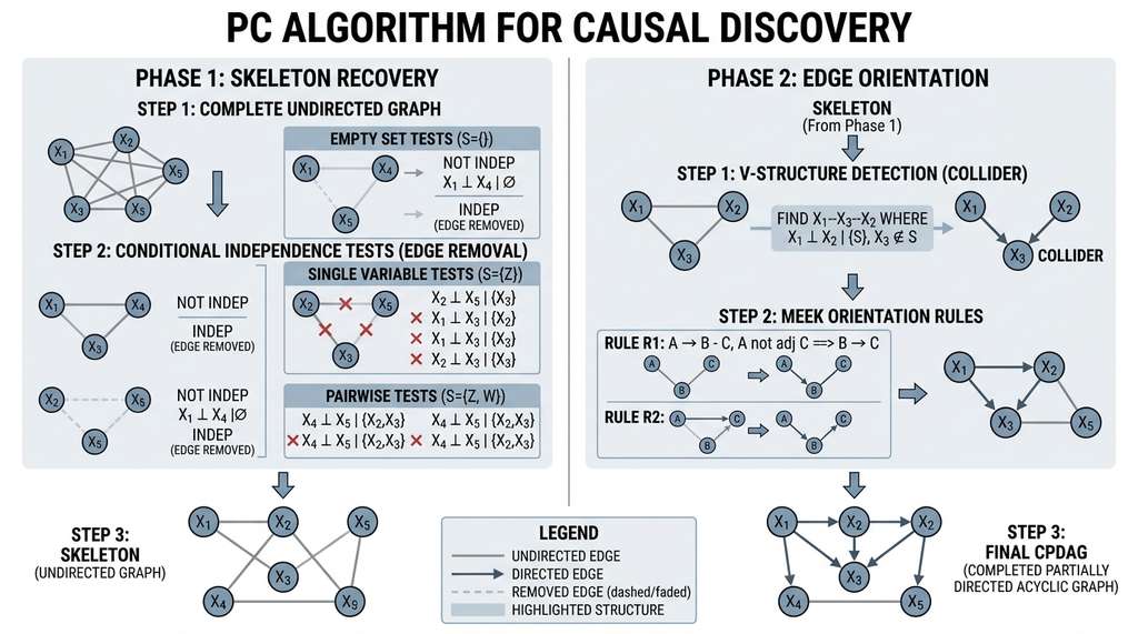
Phase 1: Skeleton recovery. Start with a complete undirected graph (every pair of variables connected). For each pair \((X, Y)\), test whether there exists a conditioning set \(Z \subseteq V \setminus \{X, Y\}\) such that \(X \perp\!\!\!\perp Y \mid Z\). If such a \(Z\) exists, remove the edge between \(X\) and \(Y\). The algorithm tests conditioning sets of increasing size: first the empty set, then single variables, then pairs, and so on. This order matters for computational efficiency, as most edges are removed by small conditioning sets.
Phase 2: Edge orientation. Apply orientation rules to direct edges where possible. First, orient v-structures: if \(X\) and \(Y\) are not adjacent but both adjacent to \(Z\), and \(Z\) was not in the separating set (the minimal conditioning set that renders \(X\) and \(Y\) independent) for \((X, Y)\), then orient \(X \to Z \leftarrow Y\). Then propagate orientations using Meek's rules, a set of four orientation constraints that direct remaining ambiguous edges by forbidding the creation of new v-structures or directed cycles (Meek, 1995).
Common Misconception
A frequent mistake is to interpret the output of PC (or GES) as "the" unique causal graph. Because these algorithms return a CPDAG, undirected edges represent genuine ambiguity: the algorithm is not uncertain or underpowered, it is telling you that multiple causal directions are equally consistent with the data. Treating an undirected edge as if it were directed in a particular way (for instance, defaulting to alphabetical or temporal order) introduces an unjustified causal claim that the data do not support.
import numpy as np
import pandas as pd
from causallearn.search.ConstraintBased.PC import pc
from causallearn.utils.cit import fisherz

# Generate data from a known causal structure:
# X1 -> X3 <- X2, X3 -> X4, X2 -> X5
np.random.seed(42)
n = 2000

X1 = np.random.normal(0, 1, n)
X2 = np.random.normal(0, 1, n)
X3 = 0.8 * X1 + 0.6 * X2 + np.random.normal(0, 0.5, n)  # Collider
X4 = 0.7 * X3 + np.random.normal(0, 0.5, n)
X5 = 0.5 * X2 + np.random.normal(0, 0.5, n)

data = np.column_stack([X1, X2, X3, X4, X5])
labels = ["X1", "X2", "X3", "X4", "X5"]

# Run the PC algorithm with Fisher's z conditional independence test
cg = pc(data, alpha=0.05, indep_test=fisherz, node_names=labels)

# Display the learned graph
print("Learned CPDAG edges:")
adj_matrix = cg.G.graph
for i in range(len(labels)):
    for j in range(i + 1, len(labels)):
        if adj_matrix[i, j] != 0 or adj_matrix[j, i] != 0:
            if adj_matrix[i, j] == -1 and adj_matrix[j, i] == 1:
                print(f"  {labels[i]} -> {labels[j]}")
            elif adj_matrix[i, j] == 1 and adj_matrix[j, i] == -1:
                print(f"  {labels[j]} -> {labels[i]}")
            elif adj_matrix[i, j] == -1 and adj_matrix[j, i] == -1:
                print(f"  {labels[i]} -- {labels[j]} (undirected)")

# Visualize the result
cg.draw_pydot_graph(labels=labels)The PC algorithm's computational complexity depends on the maximum degree of the true graph. If the maximum in-degree is \(d\), the algorithm tests conditioning sets up to size \(d\). This yields worst-case complexity of \(O(p^{d+2})\) conditional independence tests for \(p\) variables. For sparse graphs (small \(d\)), this is tractable even for thousands of variables; for dense graphs, it becomes prohibitive.
The significance level \(\alpha\) controls the skeleton density: larger \(\alpha\) removes more edges (more liberal independence testing), while smaller \(\alpha\) retains more edges (more conservative). In practice, \(\alpha = 0.01\) to \(0.05\) works well for datasets with hundreds to thousands of samples.
Step-Through: PC Algorithm on Four Variables
Trace the PC algorithm on variables \(A, B, C, D\) with 500 samples drawn from the true DAG \(A \to B \to C\), \(A \to C\), \(B \to D\).
Phase 1 (skeleton recovery). Start with all six edges: \(A{-}B\), \(A{-}C\), \(A{-}D\), \(B{-}C\), \(B{-}D\), \(C{-}D\). Test conditioning sets of size 0 first. Fisher's z gives: \(p(A \perp\!\!\!\perp D) = 0.41\) (remove \(A{-}D\)); \(p(C \perp\!\!\!\perp D) = 0.02\) (keep). All other size-0 tests yield \(p < 0.01\). Move to size-1 sets. Test \(C \perp\!\!\!\perp D \mid B\): \(p = 0.38\) (remove \(C{-}D\)). No further removals at size 1 or 2. Skeleton: \(A{-}B\), \(A{-}C\), \(B{-}C\), \(B{-}D\).
Phase 2 (orientation). Check unshielded triples. Triple \((A, C, B)\): \(A\) and \(B\) are adjacent, so no v-structure. Triple \((A, D, B)\): \(A\) and \(D\) are not adjacent; separating set for \((A, D)\) was \(\emptyset\), which does not contain \(B\), so orient \(A \to B\) and \(D \leftarrow B\). Wait: \(B\) was in no separating set? Recheck: the separating set was \(\emptyset\) (no conditioning needed). Since \(B \notin \emptyset\), orient v-structure \(A \to B \leftarrow D\)? No: \(A{-}B{-}D\) is the unshielded triple with \(A\) and \(D\) non-adjacent. The separating set of \((A, D)\) was \(\emptyset\), and \(B \notin \emptyset\), so orient \(A \to B \leftarrow D\). Apply Meek's rules: \(B \to C\) follows to avoid a new v-structure with \(A \to C\). Final CPDAG: \(A \to B \leftarrow D\), \(A \to C\), \(B \to C\). Compare to ground truth: the edge \(B \leftarrow D\) is reversed (true direction is \(B \to D\)), illustrating that a single erroneous or borderline independence test can flip an orientation.
3. The FCI Algorithm (Handling Latent Confounders)
The PC algorithm assumes causal sufficiency, where every common cause of the measured variables is itself measured. When this assumption fails (latent confounders exist), PC can produce incorrect orientations. The FCI algorithm drops this assumption and recovers a partial ancestral graph (PAG), which uses additional edge types to represent the possible presence of latent common causes.
A PAG uses three edge marks: arrowheads (\(>\)), tails (\(-\)), and circles (\(\circ\)). A circle indicates ambiguity: the mark could be either an arrowhead or a tail. For example:
- \(X \to Y\): \(X\) is a direct cause of \(Y\), and there is no latent common cause.
- \(X \leftrightarrow Y\): there is a latent common cause \(L\) with \(X \leftarrow L \to Y\) in the true DAG.
- \(X \circ\!\!\to Y\): \(X\) is either a direct cause of \(Y\) or there is a latent common cause, but we cannot distinguish which from the data.
- \(X \circ\!\!\!-\!\!\circ Y\): multiple causal relationships are consistent with the data.
from causallearn.search.ConstraintBased.FCI import fci
from causallearn.utils.cit import fisherz

# Generate data with a latent confounder
np.random.seed(42)
n = 2000

L = np.random.normal(0, 1, n)  # Latent (unmeasured) confounder
X1 = 0.7 * L + np.random.normal(0, 0.5, n)
X2 = 0.6 * L + np.random.normal(0, 0.5, n)
X3 = 0.8 * X1 + np.random.normal(0, 0.5, n)

# Only observe X1, X2, X3 (not L)
data_observed = np.column_stack([X1, X2, X3])
labels_obs = ["X1", "X2", "X3"]

# Run FCI (handles latent confounders)
G, edges = fci(data_observed, fisherz, alpha=0.05, node_names=labels_obs)

print("FCI output (PAG edges):")
adj = G.graph
for i in range(len(labels_obs)):
    for j in range(i + 1, len(labels_obs)):
        if adj[i, j] != 0 or adj[j, i] != 0:
            # Decode edge types
            marks = {-1: ">", 1: "-", 2: "o"}
            left_mark = marks.get(adj[j, i], "?")
            right_mark = marks.get(adj[i, j], "?")
            print(f"  {labels_obs[i]} {left_mark}--{right_mark} {labels_obs[j]}")

# Expected: X1 <-> X2 (bidirected, indicating latent common cause)
# X1 -> X3 (direct cause)In genomics, researchers use causal discovery to learn gene regulatory networks from expression data. A typical workflow: measure mRNA expression levels for 50 genes across 500 samples, apply FCI (because unmeasured transcription factors are almost certain), and interpret the resulting PAG. Bidirected edges (\(X \leftrightarrow Y\)) suggest co-regulation by an unmeasured factor. Directed edges (\(X \to Y\)) suggest direct regulation. Circle marks indicate uncertainty that could be resolved with additional perturbation experiments (gene knockouts or knockdowns), connecting to the experiment design methods of Chapter 46. The DREAM (Dialogue for Reverse Engineering Assessments and Methods) challenges have benchmarked causal discovery algorithms on gene regulatory networks, finding that combining constraint-based methods with expression data from perturbation experiments substantially outperforms purely observational approaches.
4. GES: Score-Based Discovery
The GES algorithm (Chickering, 2002) takes a fundamentally different approach from PC and FCI. Instead of testing conditional independencies, GES searches directly over the space of CPDAGs (equivalence classes) by greedily optimizing a scoring function, typically the Bayesian Information Criterion (BIC):
$$\text{BIC}(\mathcal{G}, \mathcal{D}) = -2 \ln L(\hat{\theta}_{\mathcal{G}}; \mathcal{D}) + k \ln n$$where \(L\) is the maximized likelihood, \(k\) is the number of free parameters in the model implied by graph \(\mathcal{G}\), and \(n\) is the sample size. The BIC penalizes model complexity, preferring simpler graphs that explain the data well.
GES proceeds in two phases:
- Forward phase: start from the empty graph. At each step, add the single edge that most improves the BIC score. Continue until no edge addition improves the score.
- Backward phase: starting from the forward phase result, delete edges one at a time, choosing the deletion that most improves BIC. Continue until no deletion improves the score.
Chickering (2002) proved that GES is consistent (meaning it recovers the correct Markov equivalence class as the sample size grows to infinity): given sufficient data from a faithful distribution, it converges to the true equivalence class. In practice, GES tends to be faster than PC on dense graphs and more robust to individual conditional independence test failures, because it considers the global fit of the entire graph rather than relying on individual pairwise tests.
from causallearn.search.ScoreBased.GES import ges

# Use the same five-variable dataset from the PC example
# X1 -> X3 <- X2, X3 -> X4, X2 -> X5
data_five = np.column_stack([X1, X2, X3, X4, X5])

# Run GES with BIC scoring
result = ges(data_five, score_func="local_score_BIC", maxP=5)

print("GES learned CPDAG:")
adj_ges = result["G"].graph
for i in range(len(labels)):
    for j in range(i + 1, len(labels)):
        if adj_ges[i, j] != 0 or adj_ges[j, i] != 0:
            if adj_ges[i, j] == -1 and adj_ges[j, i] == 1:
                print(f"  {labels[i]} -> {labels[j]}")
            elif adj_ges[i, j] == 1 and adj_ges[j, i] == -1:
                print(f"  {labels[j]} -> {labels[i]}")
            elif adj_ges[i, j] == -1 and adj_ges[j, i] == -1:
                print(f"  {labels[i]} -- {labels[j]} (undirected)")

# Compare GES and PC results
print("\nGES and PC should agree on the equivalence class.")5. LiNGAM: Exploiting Non-Gaussianity
Both PC and GES are limited to identifying equivalence classes, leaving some edge orientations ambiguous; but what if the data themselves contain a statistical signature that breaks the symmetry? The constraint-based and score-based methods above recover equivalence classes, not unique DAGs. The LiNGAM algorithm (Shimizu et al., 2006) breaks this barrier by exploiting non-Gaussian noise: under linearity and non-Gaussianity, causal direction between two variables is uniquely identifiable from observational data.
The intuition is elegant. In a linear model \(Y = \beta X + U_Y\) where \(X\) and \(U_Y\) are independent, the distribution of the residual \(Y - \beta X\) is non-Gaussian (since \(U_Y\) is non-Gaussian). If we fit the model in the wrong direction, \(X = \gamma Y + U_X\), the residual \(X - \gamma Y\) will not be independent of \(Y\) (unless the data happen to be Gaussian, where all linear models are equivalent). LiNGAM exploits this asymmetry using Independent Component Analysis (ICA), a signal-processing technique that separates a multivariate signal into maximally statistically independent components, to find the unique causal ordering.
Mental Model
Think of causal direction under non-Gaussianity like identifying the original recipe from a mixed smoothie. If someone blends mango (a distinctly flavored, non-uniform ingredient) into a base, a food chemist can separate the mango contribution from the base because mango has a recognizable chemical signature. But if someone blends plain water into plain water, you cannot tell which container was poured into which. Gaussian noise is like plain water: perfectly symmetric, so the "blending direction" is unrecoverable. Non-Gaussian noise is like mango: its distinctive distributional shape (skew, heavy tails, sharp cutoffs) leaves a fingerprint that reveals which variable was the input and which was the mixture. LiNGAM uses ICA to detect that fingerprint and determine the pouring order.
from causallearn.search.FCMBased.lingam import DirectLiNGAM

# Generate non-Gaussian data (uniform noise)
np.random.seed(42)
n = 3000

# True causal order: X1 -> X2 -> X3
e1 = np.random.uniform(-1, 1, n)  # Non-Gaussian noise
e2 = np.random.uniform(-1, 1, n)
e3 = np.random.uniform(-1, 1, n)

X1 = e1
X2 = 0.8 * X1 + e2
X3 = 0.6 * X2 + 0.3 * X1 + e3

data_lingam = np.column_stack([X1, X2, X3])
labels_lingam = ["X1", "X2", "X3"]

# Run DirectLiNGAM
model = DirectLiNGAM()
model.fit(data_lingam)

# The causal order
print(f"Discovered causal order: {[labels_lingam[i] for i in model.causal_order_]}")

# The connection strength matrix (B matrix)
print("\nConnection strength matrix B:")
print("(B[i,j] = effect of X_j on X_i)")
B = model.adjacency_matrix_
for i in range(len(labels_lingam)):
    for j in range(len(labels_lingam)):
        if abs(B[i, j]) > 0.01:
            print(f"  {labels_lingam[j]} -> {labels_lingam[i]}: {B[i,j]:.3f}")

# Compare with true values: X1->X2 = 0.8, X2->X3 = 0.6, X1->X3 = 0.3Real-World Application: Brain Connectivity Mapping
The Human Connectome Project uses DirectLiNGAM on fMRI blood-oxygen-level-dependent (BOLD) signals to infer directed connectivity between brain regions. Because BOLD signals are strongly non-Gaussian (heavy-tailed, positively skewed), LiNGAM can recover unique causal orderings that constraint-based methods cannot. Researchers at the RIKEN Center for Brain Science applied this approach to resting-state data from 200 subjects, identifying a consistent feedforward hierarchy from primary sensory cortex to prefrontal regions, with connection strengths that predicted individual differences in working memory performance.
Why does non-Gaussianity matter? The Gaussian distribution is the only distribution for which uncorrelatedness implies independence. With Gaussian noise, the models \(Y = \beta X + U_Y\) and \(X = \gamma Y + U_X\) are statistically indistinguishable (both yield Gaussian residuals independent of the regressor). With non-Gaussian noise, only the correct causal direction produces independent residuals. This is a deep result from the theory of independent component analysis: the "mixing matrix" (the causal structure) is identifiable up to permutation and scaling when the sources are non-Gaussian. In scientific data, non-Gaussianity is common (skewed distributions, heavy tails, bounded variables), making LiNGAM applicable across many domains.
6. Choosing an Algorithm
Each algorithm family has distinct strengths and limitations. Figure 31.3 summarizes the decision logic as a flowchart, and the following table details the key tradeoffs:
| Property | PC | FCI | GES | LiNGAM |
|---|---|---|---|---|
| Output | CPDAG | PAG | CPDAG | Full DAG |
| Latent confounders | No | Yes | No | No (ICA-LiNGAM: partial) |
| Linearity required | No* | No* | No* | Yes |
| Gaussianity OK | Yes | Yes | Yes | No (requires non-Gaussian) |
| Consistency | Yes | Yes | Yes | Yes |
| Scalability | Sparse graphs | Sparse graphs | Dense graphs | Moderate (\(p < 100\)) |
*PC, FCI, and GES require appropriate conditional independence tests. Fisher's z-test assumes linearity and Gaussianity; the kernel-based test (KCI) handles nonlinear relationships but is computationally expensive (\(O(n^3)\) per test). The chi-squared test handles discrete data.
A practical decision tree for choosing an algorithm (see also Figure 31.3):
- If latent confounders are plausible: use FCI.
- If all common causes are measured and noise is non-Gaussian: use LiNGAM for a unique DAG.
- If the graph is dense and Gaussian: use GES (more robust to individual test errors).
- If the graph is sparse and you want fast results: use PC.
- When in doubt: run multiple algorithms and compare. Edges that appear consistently across methods are more trustworthy than those that appear in only one.
The causal-learn library provides PC, FCI, GES, LiNGAM, and a dozen other algorithms under a unified API. What would require separate implementations of conditional independence testing, graph data structures, orientation rules, and score functions reduces to a few import statements and function calls. The library handles the graph representation (CPDAG, PAG, DAG), visualization (via pydot or matplotlib), and evaluation (structural Hamming distance for comparing learned graphs to ground truth). For production use, gCastle (Huawei's library) adds GPU-accelerated variants and differentiable structure learning methods like NOTEARS, which we discuss in the research frontier below.
7. Evaluating Discovered Graphs
Selecting an algorithm is only half the problem; once it returns a graph, you need a principled way to measure how close that graph is to the truth. When ground truth is available (simulation studies, benchmarks), we evaluate causal discovery algorithms using the Structural Hamming Distance (SHD), where SHD is the number of edge additions, deletions, and reversals needed to transform the learned graph into the true graph. An SHD of 0 means perfect recovery. Additional metrics include:
- Skeleton F1: precision and recall of the undirected skeleton (ignoring orientations).
- Arrow precision/recall: precision and recall of correctly oriented edges.
- Structural Intervention Distance (SID): counts the number of interventional distributions on which the learned and true graphs disagree. SID is more causally meaningful than SHD because it penalizes errors that affect causal inference.
from causallearn.utils.GraphUtils import GraphUtils
import numpy as np

def structural_hamming_distance(true_adj, learned_adj):
    """Compute SHD between two adjacency matrices.

    Counts edge additions, deletions, and reversals needed
    to transform learned_adj into true_adj.
    """
    p = true_adj.shape[0]
    shd = 0
    for i in range(p):
        for j in range(i + 1, p):
            true_edge = (true_adj[i, j] != 0) or (true_adj[j, i] != 0)
            learned_edge = (learned_adj[i, j] != 0) or (learned_adj[j, i] != 0)

            if true_edge and not learned_edge:
                shd += 1  # Missing edge
            elif not true_edge and learned_edge:
                shd += 1  # Extra edge
            elif true_edge and learned_edge:
                # Check orientation
                true_dir = (true_adj[i, j], true_adj[j, i])
                learned_dir = (learned_adj[i, j], learned_adj[j, i])
                if true_dir != learned_dir:
                    shd += 1  # Wrong orientation
    return shd

# Evaluate PC result against ground truth
true_adj = np.zeros((5, 5))
# True edges: X1->X3, X2->X3, X3->X4, X2->X5
true_adj[0, 2] = -1; true_adj[2, 0] = 1   # X1 -> X3
true_adj[1, 2] = -1; true_adj[2, 1] = 1   # X2 -> X3
true_adj[2, 3] = -1; true_adj[3, 2] = 1   # X3 -> X4
true_adj[1, 4] = -1; true_adj[4, 1] = 1   # X2 -> X5

pc_adj = cg.G.graph
shd = structural_hamming_distance(true_adj, pc_adj)
print(f"Structural Hamming Distance (PC): {shd}")Research Frontier
Classical algorithms like PC and GES search over discrete graph structures, limiting scalability. NOTEARS (Zheng et al., 2018) reformulated causal discovery as a continuous optimization problem by characterizing DAGs through a smooth acyclicity constraint: \(h(W) = \text{tr}(e^{W \circ W}) - d = 0\), where \(W\) is the weighted adjacency matrix, \(\circ\) denotes the element-wise (Hadamard) product, and \(d\) is the number of variables. This enables gradient-based optimization over the space of DAGs, scaling to hundreds of variables. More recently, DiffAN (Sanchez et al., 2023) introduced a differentiable approach to topological ordering that avoids the problematic acyclicity constraint entirely: it learns a causal ordering via a differentiable sorting operator and then prunes spurious edges with a variable-selection step, achieving state-of-the-art performance on the BnLearn repository (a collection of standard Bayesian network benchmarks) and SynTReN (Synthetic Transcriptional Regulatory Network, a gene-expression simulator for benchmarking) while running an order of magnitude faster than DAGMA and NOTEARS on graphs with 100+ nodes. Meanwhile, CDRL (Ke et al., 2023) applies reinforcement learning to causal discovery, training an agent to sequentially add edges while respecting acyclicity, and has shown strong results on mixed continuous-discrete data where traditional methods struggle. These methods connect to the differentiable programming paradigm of Chapter 42, where gradients flow through entire computational pipelines.
8. Practical Considerations
Running causal discovery on real scientific data requires careful attention to several practical issues:
Sample size requirements. Conditional independence tests lose power as the conditioning set grows. For PC with Fisher's z-test, a rough guideline is \(n > 10^{d/2}\) samples for a graph with maximum in-degree \(d\). (A graph with maximum in-degree 6 demands at least 1,000 samples; bump that to 10 and you need 100,000.) With 1,000 samples, conditioning sets beyond size 3 or 4 become unreliable. GES is generally more sample-efficient because it uses global scoring rather than individual tests.
Handling Heterogeneous Variables and Domain Constraints
Mixed data types. Scientific datasets often mix continuous measurements, count data, and categorical variables. Fisher's z-test handles only continuous data; the chi-squared test handles only discrete data. For mixed data, the conditional Gaussian (CG) test or kernel-based independence tests (KCI) are appropriate, though KCI scales as \(O(n^3)\) per test. An alternative is to discretize continuous variables, though this loses information.
Prior knowledge incorporation. Domain knowledge can be encoded as constraints: forbidden edges (variables that cannot be causally related), required edges (known causal relationships), and tier orderings (temporal or mechanistic ordering constraints). PC and GES in causal-learn accept these constraints, and incorporating them dramatically improves accuracy by reducing the search space.
# Incorporating prior knowledge into PC
from causallearn.search.ConstraintBased.PC import pc
from causallearn.utils.PCUtils.BackgroundKnowledge import BackgroundKnowledge

# Create background knowledge
bk = BackgroundKnowledge()

# Forbid edge: X4 cannot cause X1 (temporal ordering)
bk.add_forbidden_by_node(
    cg.G.nodes[3],  # X4
    cg.G.nodes[0],  # X1
)

# Require edge: X1 must cause X3 (domain knowledge)
bk.add_required_by_node(
    cg.G.nodes[0],  # X1
    cg.G.nodes[2],  # X3
)

# Re-run PC with background knowledge
cg_constrained = pc(
    data, alpha=0.05, indep_test=fisherz,
    node_names=labels, background_knowledge=bk
)

print("Constrained PC result:")
adj_c = cg_constrained.G.graph
for i in range(len(labels)):
    for j in range(i + 1, len(labels)):
        if adj_c[i, j] != 0 or adj_c[j, i] != 0:
            if adj_c[i, j] == -1 and adj_c[j, i] == 1:
                print(f"  {labels[i]} -> {labels[j]}")
            elif adj_c[i, j] == 1 and adj_c[j, i] == -1:
                print(f"  {labels[j]} -> {labels[i]}")
            else:
print(f" {labels[i]} -- {labels[j]}")The CausalDiscovery.org benchmarking platform hosts a running competition where researchers submit causal discovery algorithms and evaluate them on synthetic and semi-synthetic datasets with known ground truth. The leaderboard reveals a humbling pattern: no single algorithm dominates across all settings. PC tends to perform best on sparse linear Gaussian data; LiNGAM tends to lead on sparse non-Gaussian data; GES typically outperforms on dense Gaussian data; and nonlinear methods like CAM (Causal Additive Models) tend to win on nonlinear data. The practical lesson: always run multiple algorithms and trust the edges that agree.
Try It: Compare Three Algorithms on Synthetic Data
Build a short experiment that generates causal data and compares PC, GES, and LiNGAM head to head.
- Install dependencies. Run
pip install causal-learn numpy matplotlib. These are the only libraries you need. - Generate a ground-truth DAG. Create a 6-variable linear model with non-Gaussian (uniform) noise: let \(X_1\) and \(X_2\) be root causes, \(X_3 = 0.7 X_1 + 0.5 X_2 + U_3\), \(X_4 = 0.6 X_3 + U_4\), \(X_5 = 0.4 X_2 + U_5\), \(X_6 = 0.8 X_4 + 0.3 X_5 + U_6\), where each \(U_i \sim \text{Uniform}(-1, 1)\). Draw \(n = 2000\) samples.
- Run all three algorithms. Apply PC (with
fisherz, \(\alpha = 0.05\)), GES (withlocal_score_BIC), and DirectLiNGAM to the same dataset. Store each algorithm's adjacency matrix. - Compute SHD for each. Write the
structural_hamming_distancefunction from Listing 31.10 and score each learned graph against the true adjacency matrix. Print the three SHD values. - Vary sample size and plot. Repeat steps 2 through 4 for \(n \in \{200, 500, 1000, 2000, 5000\}\). Plot SHD versus \(n\) with one line per algorithm using matplotlib. Observe which algorithm converges fastest and which achieves SHD = 0 first on this non-Gaussian data.
Exercise 31.2.1
Suppose you run the PC algorithm on a dataset and obtain the skeleton \(A{-}B{-}C\) with no other edges. The separating set for \((A, C)\) is \(\{B\}\). What does the final CPDAG look like? Now change the separating set to \(\emptyset\) (i.e., \(A \perp\!\!\!\perp C\) marginally). What does the CPDAG look like in this case? Explain why the separating set determines the orientation.
Hint
A v-structure \(A \to B \leftarrow C\) is oriented when \(B\) is NOT in the separating set of \((A, C)\). If \(B\) is in the separating set, it means \(A\) and \(C\) become independent once you condition on \(B\), which is the pattern of a chain (\(A \to B \to C\) or \(A \leftarrow B \leftarrow C\)) or a fork (\(A \leftarrow B \to C\)), not a collider. Think about which d-separation pattern each case corresponds to.Lab: Causal Discovery Robustness Under Varying Noise Distributions
Goal: Observe how the choice of noise distribution affects which algorithm recovers the true causal graph most accurately.
Tools needed: Python with causal-learn, numpy, matplotlib, and scipy.stats.
Setup: Define a 5-variable linear DAG: \(X_1 \to X_2\), \(X_1 \to X_3\), \(X_2 \to X_4\), \(X_3 \to X_4\), \(X_4 \to X_5\), with edge weights drawn uniformly from \([0.5, 1.0]\). Generate \(n = 2000\) samples.
What to vary: The noise distribution for all \(U_i\) terms. Use five distributions: (1) Gaussian, (2) uniform, (3) exponential (shifted to zero mean), (4) Laplace, (5) a mixture of two Gaussians with different means. For each distribution, run PC (\(\alpha = 0.05\), Fisher's z), GES (BIC), and DirectLiNGAM. Record the SHD of each.
What to observe: Under which noise distributions does LiNGAM achieve SHD = 0 while PC and GES plateau at a nonzero SHD (stuck in the equivalence class)? Does LiNGAM degrade on Gaussian noise? Does the Gaussian mixture (which is technically non-Gaussian but close to Gaussian in shape) cause LiNGAM to struggle? Plot a grouped bar chart: noise type on the x-axis, SHD on the y-axis, one bar group per algorithm. This reveals the practical boundary of the non-Gaussianity assumption.
Exercises
- (Conceptual) Consider a dataset with five variables where the true DAG is \(A \to B \to C\), \(A \to D\), \(D \to C\), \(B \to E\). Draw the CPDAG (Markov equivalence class). Which edges are directed and which are undirected? Identify all v-structures. Now suppose the noise terms are all uniform (non-Gaussian). Does LiNGAM recover the full DAG? Why?
- (Coding) Generate data from a 10-variable linear Gaussian DAG (use a random sparse adjacency matrix with density 0.3). Run PC, GES, and LiNGAM on the same data and compare their SHD scores. Repeat for sample sizes \(n \in \{200, 500, 1000, 5000\}\) and plot SHD versus \(n\) for all three algorithms. At what sample size does each algorithm's SHD stabilize? What happens to LiNGAM on Gaussian data?
- (Analysis) Download the Sachs et al. (2005) protein signaling dataset (available in causal-learn's example datasets). Run FCI on this data and interpret the PAG. Which edges are bidirected (suggesting latent confounders)? Compare your result to the expert-curated network published in the original paper. Discuss: where does the algorithm agree with domain knowledge, and where does it disagree?
What's Next
Causal discovery gives us the graph; now we need to quantify the causal effects encoded in it. In Section 31.3: Treatment Effect Estimation, we move from structure to strength: estimating the average treatment effect (ATE), the average treatment effect on the treated (ATT), and the conditional average treatment effect (CATE) using modern semiparametric methods. Double machine learning and meta-learners combine the flexibility of ML models with the rigor of causal identification, and sensitivity analysis with E-values quantifies robustness to unmeasured confounding.