Prerequisites
Section 31.1 introduced the structural causal model formalism, the do-operator, and the backdoor criterion for identification. Section 31.2 covered learning causal graphs from data. This section addresses the quantitative question: given a causal graph and observational data, how large is the causal effect? Prerequisites include the backdoor adjustment formula, potential outcomes, and the ignorability assumption. The estimation methods below use logistic regression and random forests from Chapter 5.
Treatment effect estimation bridges the gap between causal identification (can we compute the effect?) and statistical estimation (what is the effect, and how precisely do we know it?). This section covers three layers of increasing richness: the average treatment effect (ATE), which summarizes the population-level impact; the average treatment effect on the treated (ATT), which focuses on those who actually received treatment; and the conditional average treatment effect (CATE), which reveals how the effect varies across subpopulations. Modern semiparametric methods (double machine learning (DML), meta-learners) let us use flexible ML models for nuisance estimation while preserving valid confidence intervals for the causal parameter. E-value sensitivity analysis then quantifies how robust our conclusions are to unmeasured confounding.
1. The Estimands: ATE, ATT, CATE
A new drug cuts hospitalizations in half for patients over 65, yet it has zero measurable benefit for patients under 40. Reporting only the average effect would greenlight the drug for everyone or reject it for everyone, both wrong answers. Separating "how large is the effect overall?" from "who benefits most?" requires three distinct estimands, each answering a different scientific question about the same treatment.
Using the potential outcomes notation from Section 31.1, we define these three estimands for a binary treatment \(T \in \{0, 1\}\):
The Average Treatment Effect (ATE) is the expected difference in potential outcomes across the entire population:
$$\text{ATE} = E[Y(1) - Y(0)] = E[Y(1)] - E[Y(0)]$$The Average Treatment Effect on the Treated (ATT) restricts the comparison to units that actually received treatment:
$$\text{ATT} = E[Y(1) - Y(0) \mid T = 1] = E[Y(1) \mid T = 1] - E[Y(0) \mid T = 1]$$The ATT is often the policy-relevant quantity: it answers "how much did the treatment help those who received it?" The second term, \(E[Y(0) \mid T = 1]\), is the expected outcome the treated group would have had under control, which is counterfactual and must be estimated.
The Conditional Average Treatment Effect (CATE) captures treatment effect heterogeneity by conditioning on covariates:
$$\tau(x) = E[Y(1) - Y(0) \mid X = x]$$CATE is a function, not a number. It tells us which subpopulations benefit most (or are harmed) by the treatment. In personalized medicine, CATE estimation drives treatment recommendations: give the drug to patients with \(\tau(x) > 0\) and withhold it from those with \(\tau(x) < 0\). CATE estimation is the most challenging task because it requires modeling a function over the covariate space, not estimating a single scalar. In short: the right question is never "does the treatment work?" but "for whom does it work, and by how much?"
Choosing between ATE, ATT, and CATE is not a statistical decision; it is a scientific one. ATE answers: "if we treated everyone, what would the average benefit be?" ATT answers: "did the treatment help those who received it?" CATE answers: "who benefits most?" A drug with ATE = 0 might still have \(\tau(x) > 0\) for a subpopulation and \(\tau(x) < 0\) for another, meaning it helps some patients and harms others. Reporting only the ATE would hide this heterogeneity. Conversely, a policy maker deciding whether to universally deploy a fertilizer needs the ATE, not the CATE. The estimand must match the scientific question before any estimation begins.
The treatment effect estimation pipeline, shown in Figure 31.6, follows a common structure across all the methods in this section: fit nuisance models (a propensity model for treatment assignment and an outcome model for the response), feed their predictions into an estimator formula that isolates the causal effect, and then stress-test the result with sensitivity analysis or refutation tests.
2. Inverse Propensity Weighting
The simplest approach to ATE estimation is the Horvitz-Thompson estimator, also called inverse propensity weighting (IPW). The key idea: in observational data, treatment assignment is non-random, so naive comparisons of treated and control groups are biased. IPW corrects this by reweighting each observation by the inverse of its probability of receiving the treatment it actually received.
The propensity score is the probability of receiving treatment given covariates:
$$e(x) = P(T = 1 \mid X = x)$$A propensity score is a single number between 0 and 1 that summarizes how likely a unit was to receive treatment, given all observed characteristics. This scalar reduces a high-dimensional covariate adjustment problem to a one-dimensional balancing problem. Instead of matching on every covariate individually, you balance on this single number. To compute it, fit a classification model (logistic regression, gradient boosting, or any probabilistic classifier) that predicts treatment assignment from covariates, then use the predicted probabilities as scores. Use propensity scores when many covariates make direct matching impractical. Use regression adjustment when you have few covariates and prefer to model the outcome directly. Use doubly robust methods (Section 3 below) when you want protection against misspecification in either model.
The IPW estimator for the ATE is:
$$\hat{\tau}_{\text{IPW}} = \frac{1}{n} \sum_{i=1}^{n} \left[ \frac{T_i Y_i}{e(X_i)} - \frac{(1 - T_i) Y_i}{1 - e(X_i)} \right]$$The intuition: a treated unit with propensity score \(e(x) = 0.9\) was very likely to be treated anyway, so it gets weight \(1/0.9 \approx 1.1\); it does not teach us much about what would happen if we treated a randomly chosen unit. A treated unit with \(e(x) = 0.2\) was unlikely to be treated, so it gets weight \(1/0.2 = 5\); it is more "informative" about the treatment effect because it resembles the control population.
Common Misconception
A frequent misconception is that IPW (or any method that adjusts for observed covariates) fully eliminates confounding bias. It does not. IPW corrects for measured confounders only. If an unmeasured variable influences both treatment assignment and the outcome, the reweighted estimate remains biased regardless of how accurately you model the propensity score. Adjusting for observed covariates is necessary but never sufficient to guarantee a causal interpretation; that guarantee requires the untestable ignorability assumption (the assumption that treatment assignment is independent of potential outcomes conditional on observed covariates, written \(T \perp\!\!\!\perp Y(0), Y(1) \mid X\)), which is why sensitivity analysis (Section 6) is essential.
import numpy as np
import pandas as pd
from sklearn.linear_model import LogisticRegression

np.random.seed(42)
n = 5_000

# Simulate observational data with confounding
X1 = np.random.normal(0, 1, n)  # Age (standardized)
X2 = np.random.normal(0, 1, n)  # Severity (standardized)

# Treatment assignment depends on confounders
propensity_true = 1 / (1 + np.exp(-(0.5 * X1 + 0.8 * X2)))
T = np.random.binomial(1, propensity_true)

# Outcome with heterogeneous treatment effect
Y = 2 * T + 0.5 * X1 - 0.3 * X2 + 0.4 * T * X1 + np.random.normal(0, 1, n)

data = pd.DataFrame({"X1": X1, "X2": X2, "T": T, "Y": Y})

# Naive estimate (biased)
naive = data[data.T == 1]["Y"].mean() - data[data.T == 0]["Y"].mean()
print(f"Naive ATE: {naive:.3f}")  # Biased upward

# IPW estimate
lr = LogisticRegression()
lr.fit(data[["X1", "X2"]], data["T"])
e_hat = lr.predict_proba(data[["X1", "X2"]])[:, 1]

# Clip propensity scores to avoid extreme weights
e_hat = np.clip(e_hat, 0.05, 0.95)

ipw_ate = np.mean(T * Y / e_hat - (1 - T) * Y / (1 - e_hat))
print(f"IPW ATE: {ipw_ate:.3f}")

# True ATE: E[2 + 0.4*X1] = 2 + 0.4*E[X1] = 2 + 0 = 2.0
print(f"True ATE: 2.000")IPW has a well-known weakness: when propensity scores are close to 0 or 1, the weights become extreme, inflating variance. This is called positivity violation or practical non-overlap. Clipping propensity scores (as in the code above) is the simplest remedy, but it introduces bias. A more principled solution is the doubly robust estimator, which combines propensity weighting with outcome regression.
Step-Through: IPW Weight Calculation
Trace through the IPW estimator with five observations. Suppose we have:
| Unit | \(T_i\) | \(Y_i\) | \(e(X_i)\) |
|---|---|---|---|
| 1 | 1 | 8 | 0.80 |
| 2 | 1 | 6 | 0.30 |
| 3 | 0 | 4 | 0.70 |
| 4 | 0 | 5 | 0.20 |
| 5 | 1 | 7 | 0.50 |
For each unit, compute \(T_i Y_i / e(X_i) - (1 - T_i) Y_i / (1 - e(X_i))\):
- Unit 1 (treated): \(1 \times 8 / 0.80 - 0 = 10.0\)
- Unit 2 (treated): \(1 \times 6 / 0.30 - 0 = 20.0\) (low propensity, large weight)
- Unit 3 (control): \(0 - 1 \times 4 / 0.30 = -13.33\)
- Unit 4 (control): \(0 - 1 \times 5 / 0.80 = -6.25\)
- Unit 5 (treated): \(1 \times 7 / 0.50 - 0 = 14.0\)
\(\hat{\tau}_{\text{IPW}} = (10.0 + 20.0 - 13.33 - 6.25 + 14.0) / 5 = 4.88\). Notice that Unit 2, a treated unit with low propensity (\(e = 0.30\)), received the largest weight (20.0) because it is the most "surprising" treatment assignment. This is exactly the IPW mechanism: unlikely-to-be-treated units that were treated carry more information about the causal effect.
3. Doubly Robust Estimation
The augmented inverse propensity weighted (AIPW) estimator, also called the doubly robust estimator, combines outcome regression \(\hat{\mu}(t, x) = \hat{E}[Y \mid T = t, X = x]\) with propensity weighting:
$$\hat{\tau}_{\text{AIPW}} = \frac{1}{n} \sum_{i=1}^{n} \left[ \hat{\mu}(1, X_i) - \hat{\mu}(0, X_i) + \frac{T_i (Y_i - \hat{\mu}(1, X_i))}{e(X_i)} - \frac{(1 - T_i)(Y_i - \hat{\mu}(0, X_i))}{1 - e(X_i)} \right]$$The "doubly robust" property: the estimator is consistent if either the propensity score model \(e(x)\) or the outcome model \(\hat{\mu}(t, x)\) is correctly specified. You get two chances to get it right, not one. In a benchmark by Naimi et al. (2021) comparing 23 estimators across 3,600 simulated scenarios, the doubly robust estimators were the only ones that maintained low bias in nearly all settings, even when one nuisance model was severely misspecified. If both models are correct, AIPW achieves the semiparametric efficiency bound (the lowest possible asymptotic variance attainable by any regular estimator that does not assume a fully parametric model for the data-generating process).
Mental Model
Think of double robustness like navigating to a friend's house using both a GPS and written directions. If the GPS has accurate maps but a weak signal (the propensity model is right, the outcome model is wrong), you still arrive. If the GPS signal drops entirely but the written directions are correct (the outcome model is right, the propensity model is wrong), you also arrive. You only get lost if both the GPS and the written directions are simultaneously wrong. The AIPW estimator works the same way: the propensity model corrects the residual errors of the outcome model, and vice versa, so you need both to fail for the estimate to be biased. This is not just a convenience; it is a structural property of how the two correction terms cancel each other's mistakes in the formula above.
from sklearn.ensemble import GradientBoostingRegressor, GradientBoostingClassifier

# Outcome models: E[Y | T=t, X]
mu1_model = GradientBoostingRegressor(n_estimators=100, max_depth=3)
mu0_model = GradientBoostingRegressor(n_estimators=100, max_depth=3)

treated = data[data.T == 1]
control = data[data.T == 0]

mu1_model.fit(treated[["X1", "X2"]], treated["Y"])
mu0_model.fit(control[["X1", "X2"]], control["Y"])

mu1_hat = mu1_model.predict(data[["X1", "X2"]])
mu0_hat = mu0_model.predict(data[["X1", "X2"]])

# Propensity model
ps_model = GradientBoostingClassifier(n_estimators=100, max_depth=3)
ps_model.fit(data[["X1", "X2"]], data["T"])
e_hat_gb = np.clip(ps_model.predict_proba(data[["X1", "X2"]])[:, 1], 0.05, 0.95)

# AIPW estimator
aipw_scores = (
    (mu1_hat - mu0_hat)
    + T * (Y - mu1_hat) / e_hat_gb
    - (1 - T) * (Y - mu0_hat) / (1 - e_hat_gb)
)
aipw_ate = aipw_scores.mean()
aipw_se = aipw_scores.std() / np.sqrt(n)

print(f"AIPW ATE: {aipw_ate:.3f} (SE: {aipw_se:.3f})")
print(f"95% CI: [{aipw_ate - 1.96*aipw_se:.3f}, {aipw_ate + 1.96*aipw_se:.3f}]")
print(f"True ATE: 2.000")A pharmaceutical company studies whether a new anti-inflammatory drug reduces joint pain scores. Observational data from electronic health records show that older patients and those with higher baseline inflammation are more likely to receive the drug (confounding by indication). The company runs DML (introduced in Section 4 below) with gradient boosting for both nuisance models, using age, baseline inflammation, BMI, and comorbidity count as covariates. The overall ATE is 1.2 points on a 10-point pain scale (\(p < 0.001\)). But the CATE analysis reveals dramatic heterogeneity: patients with high baseline inflammation (\(> 2\) SD above mean) show CATE = 3.1 points, while patients with low baseline inflammation show CATE = 0.3 points (not significant). This heterogeneity, invisible in the ATE, directly informs personalized treatment guidelines. The analysis connects to the biology and medicine applications in Chapter 48.
4. Double Machine Learning
When analysts plug flexible ML models into the IPW or AIPW formulas without additional safeguards, the resulting confidence intervals can be wildly overconfident because the ML models' own estimation error leaks into the causal estimate. Double machine learning was designed to solve exactly this problem, ensuring that the statistical guarantees on the treatment effect remain valid no matter how complex the nuisance models (auxiliary models whose parameters are not of scientific interest but must be estimated as intermediate steps, such as the propensity score and the conditional outcome mean) become.
Double Machine Learning (DML), introduced by Chernozhukov et al. (2018), provides a rigorous framework for using arbitrary ML models (random forests, neural networks, gradient boosting) for nuisance estimation while preserving \(\sqrt{n}\)-consistent, asymptotically normal inference on the causal parameter. The key innovations are:
- Neyman orthogonality (a property requiring that the moment condition used to identify the causal parameter has zero first-order sensitivity to perturbations in the nuisance estimates): construct a moment condition for the causal parameter that is locally insensitive to errors in the nuisance estimates. This allows the nuisance models to converge at slower-than-\(\sqrt{n}\) rates (as ML models typically do) without contaminating the causal estimate.
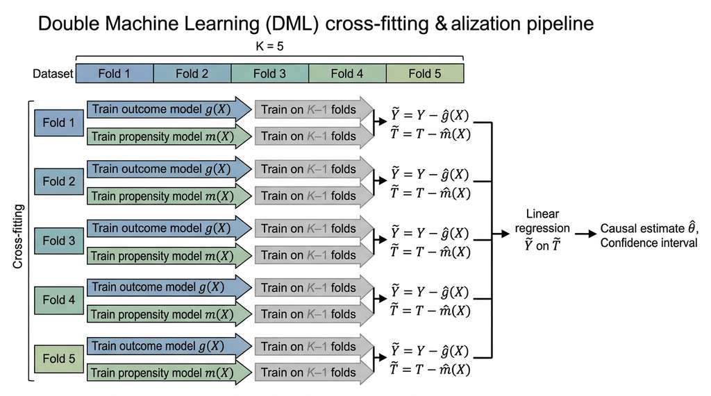
- Cross-fitting: split the data into \(K\) folds. For each fold, estimate nuisance parameters on the other \(K - 1\) folds and compute the causal estimate on the held-out fold. This avoids overfitting bias from using the same data for nuisance estimation and causal inference.
The partially linear model \(Y = \theta T + g(X) + U\), \(T = m(X) + V\) illustrates the DML recipe. The causal parameter \(\theta\) is the treatment effect. The functions \(g(X) = E[Y \mid X]\) and \(m(X) = E[T \mid X]\) are nuisance parameters estimated by ML. The DML estimator:
- Residualize \(Y\) against \(X\): compute \(\tilde{Y} = Y - \hat{g}(X)\).
- Residualize \(T\) against \(X\): compute \(\tilde{T} = T - \hat{m}(X)\).
- Regress \(\tilde{Y}\) on \(\tilde{T}\): \(\hat{\theta} = (\tilde{T}^\top \tilde{T})^{-1} \tilde{T}^\top \tilde{Y}\).
Checkpoint
So far: DML uses two ideas to let flexible ML models estimate causal effects without corrupting inference. Neyman orthogonality ensures the causal estimate is insensitive to small errors in the nuisance models, and cross-fitting prevents overfitting by never using the same data for nuisance estimation and causal parameter estimation.
The residualization "partials out" the confounders, isolating the variation in \(T\) that is not explained by \(X\), which is the variation that is as-good-as-random under the ignorability assumption. This is a nonparametric generalization of the Frisch-Waugh-Lovell theorem (a classical econometrics result stating that the coefficient on one regressor in a multivariate OLS regression equals the coefficient from a simple regression of the residualized outcome on the residualized regressor, after partialing out all other covariates). Figure 31.3.1 illustrates Double Machine Learning cross-fitting and residualization pipeline.
from econml.dml import LinearDML
from sklearn.ensemble import RandomForestRegressor, RandomForestClassifier

# Double ML with EconML
dml = LinearDML(
    model_y=RandomForestRegressor(n_estimators=200, max_depth=5, min_samples_leaf=10),
    model_t=RandomForestClassifier(n_estimators=200, max_depth=5, min_samples_leaf=10),
    cv=5,  # 5-fold cross-fitting
    random_state=42,
)

X_covariates = data[["X1", "X2"]].values
T_treatment = data["T"].values
Y_outcome = data["Y"].values

dml.fit(Y_outcome, T_treatment, X=X_covariates)

# ATE with confidence interval
ate = dml.ate()
ate_interval = dml.ate_interval(alpha=0.05)
print(f"DML ATE: {ate:.3f}")
print(f"95% CI: [{ate_interval[0]:.3f}, {ate_interval[1]:.3f}]")
print(f"True ATE: 2.000")

# CATE: treatment effect as a function of covariates
# Predict CATE for specific covariate values
test_points = np.array([[0, 0], [1, 0], [-1, 0], [0, 1]])
cate_predictions = dml.effect(test_points)
cate_intervals = dml.effect_interval(test_points, alpha=0.05)

print("\nCate predictions:")
for i, (x, tau, ci) in enumerate(zip(test_points, cate_predictions, zip(*cate_intervals))):
print(f" X={x}: CATE={tau:.3f}, 95% CI=[{ci[0]:.3f}, {ci[1]:.3f}]")5. Meta-Learners for CATE
DML provides a principled framework for estimating both ATE and CATE, but it assumes a specific partially linear or interactive model structure; when the goal is purely to estimate a flexible CATE function without committing to a particular structural form, a family of lighter-weight strategies called meta-learners offers complementary alternatives.
Meta-learners are a family of strategies for estimating CATE by combining base ML models in specific ways. The three most common meta-learners are:
The Three Core Meta-Learners
T-learner: fit separate outcome models for treated (\(\hat{\mu}_1(x)\)) and control (\(\hat{\mu}_0(x)\)) groups. The CATE estimate is \(\hat{\tau}(x) = \hat{\mu}_1(x) - \hat{\mu}_0(x)\). Simple but can suffer from regularization bias (systematic error introduced when a model's complexity penalty shrinks the estimated treatment effect toward zero) when the treatment and control groups have different sample sizes or covariate distributions.
S-learner: fit a single outcome model \(\hat{\mu}(t, x)\) that includes treatment as a feature. The CATE estimate is \(\hat{\tau}(x) = \hat{\mu}(1, x) - \hat{\mu}(0, x)\). Can underestimate heterogeneity because regularization may shrink the treatment effect toward zero if it is small relative to the main effects.
X-learner (Kunzel et al., 2019): a two-stage procedure that is especially effective when the treated and control groups are imbalanced. Stage 1: fit T-learner models. Stage 2: impute individual treatment effects by applying each group's model to the other group's data. Stage 3: combine the imputed effects using a propensity-score-weighted average.
from econml.metalearners import TLearner, SLearner, XLearner
from sklearn.ensemble import GradientBoostingRegressor

# T-Learner
t_learner = TLearner(
    models=GradientBoostingRegressor(n_estimators=200, max_depth=4)
)
t_learner.fit(Y_outcome, T_treatment, X=X_covariates)

# S-Learner
s_learner = SLearner(
    overall_model=GradientBoostingRegressor(n_estimators=200, max_depth=4)
)
s_learner.fit(Y_outcome, T_treatment, X=X_covariates)

# X-Learner
x_learner = XLearner(
    models=GradientBoostingRegressor(n_estimators=200, max_depth=4),
    propensity_model=LogisticRegression(),
)
x_learner.fit(Y_outcome, T_treatment, X=X_covariates)

# Compare CATE estimates at test points
print("CATE comparison at X1=1, X2=0:")
test_x = np.array([[1.0, 0.0]])
print(f"  T-learner: {t_learner.effect(test_x)[0]:.3f}")
print(f"  S-learner: {s_learner.effect(test_x)[0]:.3f}")
print(f"  X-learner: {x_learner.effect(test_x)[0]:.3f}")
print(f"  True CATE: {2 + 0.4 * 1.0:.3f}")  # tau(x) = 2 + 0.4*X1

# Population-level CATE distribution
cate_t = t_learner.effect(X_covariates)
cate_s = s_learner.effect(X_covariates)
cate_x = x_learner.effect(X_covariates)

print(f"\nPopulation CATE statistics:")
print(f"  T-learner: mean={cate_t.mean():.3f}, std={cate_t.std():.3f}")
print(f"  S-learner: mean={cate_s.mean():.3f}, std={cate_s.std():.3f}")
print(f"  X-learner: mean={cate_x.mean():.3f}, std={cate_x.std():.3f}")
EconML provides T-learner, S-learner, X-learner, doubly robust learner, causal forests
(Athey and Wager, 2019), and the DRLearner, all with a unified fit/effect/effect_interval
API. The library handles cross-fitting, propensity estimation, and confidence interval
construction internally. What would require implementing the full X-learner two-stage
procedure from scratch (separate model fits, counterfactual imputation, propensity-weighted
combination) reduces to three lines of code. EconML also integrates with DoWhy for the
identification step, creating a seamless model-identify-estimate-refute pipeline.
6. Sensitivity Analysis with E-Values
The estimators above (IPW, AIPW, DML, and meta-learners) all produce point estimates and confidence intervals, but every one of them depends on the assumption that all relevant confounders have been measured; the next question is how to gauge whether that assumption could plausibly fail.
Every observational causal analysis rests on the assumption that all confounders are measured (ignorability). This assumption is untestable: we can never rule out the existence of an unmeasured confounder that biases our estimate. Sensitivity analysis quantifies how strong such an unmeasured confounder would need to be to explain away the observed effect.
The E-value (VanderWeele and Ding, 2017) provides an intuitive measure of robustness. For an observed risk ratio (the ratio of the probability of the outcome in the treated group to its probability in the control group, written \(\text{RR} = P(Y=1 \mid T=1) / P(Y=1 \mid T=0)\)) \(\text{RR}\), the E-value is:
$$E\text{-value} = \text{RR} + \sqrt{\text{RR} \times (\text{RR} - 1)}$$The E-value is the minimum association strength (on the risk ratio scale) that an unmeasured confounder would need with both treatment and outcome, beyond measured covariates, to fully explain away the observed effect. Large E-values signal robustness; small ones (close to 1) warn that even a weak unmeasured confounder could overturn the conclusion.
import numpy as np

def compute_e_value(risk_ratio: float, ci_bound: float = None) -> dict:
    """Compute the E-value for an observed risk ratio.

    Parameters
    ----------
    risk_ratio : float
        Observed risk ratio (must be >= 1; if < 1, invert it).
    ci_bound : float, optional
        The confidence interval bound closest to 1.0.

    Returns
    -------
    dict with E-value for point estimate and CI bound.
    """
    if risk_ratio < 1:
        risk_ratio = 1 / risk_ratio  # Work with RR >= 1

    e_point = risk_ratio + np.sqrt(risk_ratio * (risk_ratio - 1))

    result = {"e_value_point": e_point}

    if ci_bound is not None:
        if ci_bound < 1:
            ci_bound = 1 / ci_bound
        if ci_bound <= 1.0:
            result["e_value_ci"] = 1.0  # CI crosses null
        else:
            result["e_value_ci"] = ci_bound + np.sqrt(ci_bound * (ci_bound - 1))

    return result

# Example: drug reduces mortality with RR = 0.6, 95% CI [0.45, 0.80]
result = compute_e_value(risk_ratio=0.6, ci_bound=0.80)
print(f"E-value for point estimate (RR=0.6): {result['e_value_point']:.2f}")
print(f"E-value for CI bound (RR=0.80):      {result['e_value_ci']:.2f}")
print()
print("Interpretation: an unmeasured confounder would need to be associated")
print(f"with both treatment and outcome by a factor of {result['e_value_point']:.1f}")
print("(beyond measured covariates) to explain away the point estimate.")
print(f"A factor of {result['e_value_ci']:.1f} would move the CI to include the null.")Reporting a causal effect without sensitivity analysis is like reporting a measurement without an uncertainty estimate: the number is meaningless without context about its reliability. The E-value provides that context by translating the abstract worry "what if there is unmeasured confounding?" into a concrete quantitative statement: "the result would be overturned only if an unmeasured confounder existed that was associated with both treatment and outcome by a risk ratio of at least \(X\)." Researchers and reviewers can then judge whether such a confounder is plausible in their domain. For drug safety studies, regulatory agencies increasingly require sensitivity analysis alongside point estimates.
7. DoWhy Refutation Tests
E-values quantify robustness to a single hypothetical unmeasured confounder, but a causal estimate can also be fragile in other ways: it might depend on a few influential observations, collapse under a different covariate adjustment set, or vanish when the treatment variable is shuffled. A broader suite of stress tests can probe these failure modes systematically.
DoWhy (as of 2024, v0.11+ uses a redesigned graph-first API; the legacy API shown below still works but is deprecated) implements a battery of refutation tests that stress-test causal estimates by checking whether the estimate behaves as expected under controlled perturbations. These are not tests of statistical significance; they are tests of causal model specification. The main refutation methods are:
- Placebo treatment: replace the real treatment with a random variable. If the causal model is correct, the estimated effect should be approximately zero.
- Random common cause: add a random variable as an additional confounder. If the original adjustment set was sufficient, the estimate should not change substantially.
- Data subset: re-estimate on a random subset of the data. The estimate should remain stable (within sampling variability).
- Unobserved common cause: simulate the effect of an unmeasured confounder with specified strength. Quantifies how sensitive the estimate is to omitted variable bias.
import dowhy
from dowhy import CausalModel

# Set up the DoWhy model
df = pd.DataFrame({"X1": X1, "X2": X2, "T": T, "Y": Y})

model = CausalModel(
    data=df,
    treatment="T",
    outcome="Y",
    common_causes=["X1", "X2"],
)

identified = model.identify_effect()
estimate = model.estimate_effect(
    identified,
    method_name="backdoor.econml.dml.DML",
    method_params={
        "init_params": {
            "model_y": GradientBoostingRegressor(n_estimators=100),
            "model_t": GradientBoostingClassifier(n_estimators=100),
            "cv": 3,
        },
        "fit_params": {},
    },
)
print(f"Estimated ATE: {estimate.value:.3f}")

# Refutation 1: Placebo treatment
refute_placebo = model.refute_estimate(
    identified, estimate,
    method_name="placebo_treatment_refuter",
    placebo_type="permute",
    num_simulations=100,
)
print(f"\nPlacebo refutation:")
print(f"  Estimated effect with placebo: {refute_placebo.new_effect:.3f}")
print(f"  p-value: {refute_placebo.refutation_result['p_value']:.4f}")

# Refutation 2: Random common cause
refute_random = model.refute_estimate(
    identified, estimate,
    method_name="random_common_cause",
    num_simulations=100,
)
print(f"\nRandom common cause refutation:")
print(f"  Estimated effect with random confounder: {refute_random.new_effect:.3f}")

# Refutation 3: Data subset
refute_subset = model.refute_estimate(
    identified, estimate,
    method_name="data_subset_refuter",
    subset_fraction=0.8,
    num_simulations=100,
)
print(f"\nSubset refutation:")
print(f" Estimated effect on 80% subset: {refute_subset.new_effect:.3f}")Real-World Application: Microsoft's Causal Impact of LinkedIn Features
Microsoft's ExP (Experimentation Platform) team uses EconML's DML and causal forest estimators to measure the heterogeneous effect of LinkedIn product changes (such as "People You May Know" algorithm updates) on user engagement. Because not all users can be randomized into A/B tests (some features roll out by region or device), the team applies doubly robust CATE estimation on observational logs, conditioning on hundreds of user-level covariates. The CATE surfaces reveal that algorithm changes often help new users substantially while having near-zero effect on power users, guiding targeted rollout decisions that would be invisible under a single ATE number.
Recent work pushes treatment effect estimation beyond the methods covered here. Chernozhukov et al. (2024) introduced Automatic Debiased Machine Learning (AutoDML), which automates the construction of Neyman-orthogonal moment conditions for a broad class of causal parameters, removing the need for analysts to hand-derive the debiasing correction for each new estimand. Separately, Shi et al. (2024) reported that large language model embeddings of unstructured clinical notes can serve as high-dimensional proxies for unmeasured confounders, in some cases reducing residual bias in observational studies where structured covariates alone are insufficient. Their CausalBERT framework fine-tunes a pretrained transformer to jointly predict treatment and outcome; on several electronic health record benchmarks it achieved tighter CATE intervals than traditional covariate-based approaches, though the generality of these gains across different clinical domains remains an open question. These directions suggest that the next generation of causal estimation tools will combine flexible debiasing theory with representation learning from unstructured data sources.
In a 2021 simulation study, Naimi et al. compared 23 causal estimators across 3,600 data-generating processes. The doubly robust estimators (AIPW and targeted maximum likelihood estimation (TMLE)) were the only ones that maintained low bias across nearly all settings, even when one of the two nuisance models was badly misspecified. The IPW estimator was unbiased when the propensity model was correct but catastrophically biased otherwise. The outcome regression estimator showed the opposite pattern. The doubly robust estimator was, in the authors' words, "never the worst and often the best." If you must pick one estimator for a paper, pick AIPW.
Try It: End-to-End Treatment Effect Estimation on Simulated Data
Build a complete causal estimation pipeline from scratch using only NumPy, scikit-learn, and EconML.
- Simulate a confounded dataset. Generate 5,000 observations with two covariates (\(X_1\), \(X_2\)), a binary treatment assigned via a logistic model that depends on both covariates (creating confounding), and an outcome \(Y = 3T + X_1 - 0.5 X_2 + T \cdot X_1 + \varepsilon\). Record the true ATE (3.0) and true CATE function \(\tau(x) = 3 + X_1\).
- Estimate propensity scores and run IPW. Fit a logistic regression to predict \(T\) from \((X_1, X_2)\). Clip scores to \([0.05, 0.95]\). Compute the IPW estimate. Compare it to the naive difference in group means and note the bias correction.
- Run the AIPW estimator. Fit two gradient boosting regressors (one for treated outcomes, one for control outcomes) and combine them with the propensity scores in the AIPW formula. Compute the 95% confidence interval using the influence-function standard error.
- Estimate heterogeneous effects with DML. Use
econml.dml.LinearDMLwith random forest nuisance models and 5-fold cross-fitting. Plot the estimated CATE against \(X_1\) and overlay the true CATE line \(\tau(x) = 3 + X_1\). Verify that the slope is recovered. - Compute E-values. Convert your ATE estimate and its confidence interval to the risk-ratio scale (using the formula \(\text{RR} \approx \exp(\hat{\tau} / \text{SD}(Y_0))\)), then compute E-values for both the point estimate and the confidence interval bound. Interpret: how strong would an unmeasured confounder need to be to nullify your finding?
Exercise 31.3.1
You run an IPW analysis and obtain an ATE estimate of 4.2. You then clip propensity scores from \([0.01, 0.99]\) to \([0.10, 0.90]\) and the estimate drops to 3.1. Finally, you clip to \([0.20, 0.80]\) and the estimate drops further to 2.5. What does this pattern tell you about your data? Would you trust the original estimate? Explain what is happening mechanically and what assumption is likely being violated.
Hint
Consider which observations receive the largest IPW weights and what happens when you remove them. If the estimate is highly sensitive to a handful of units with extreme propensity scores (near 0 or 1), those units are in a region of poor overlap between the treated and control covariate distributions. This is a positivity violation: there exist covariate values where treatment assignment is nearly deterministic, so the counterfactual outcome is being extrapolated from very few (or zero) comparable units in the opposite group. The instability across clipping thresholds is a diagnostic signal that the ATE may not be reliably identified in your data without stronger modeling assumptions.
Lab: Propensity Score Overlap and Estimator Breakdown
Goal: Observe how treatment effect estimators degrade as propensity score overlap weakens, and learn to diagnose positivity violations before they corrupt your estimates.
Tools: Python with NumPy, scikit-learn, EconML, and matplotlib (about 20 minutes).
Protocol: Simulate a dataset with two covariates, a true ATE of 2.0, and treatment assignment governed by a logistic model \(P(T=1 \mid X) = \text{logit}^{-1}(\gamma \cdot X_1)\). Start with \(\gamma = 0.5\) (good overlap) and increase it through \(\{0.5, 1.0, 2.0, 3.0, 5.0\}\) (progressively worse overlap). For each value of \(\gamma\), estimate the ATE using IPW, AIPW, and DML. Plot the propensity score distributions for treated and control groups side by side, and plot each estimator's ATE estimate (with 95% CI) against the true value.
What to vary: The overlap parameter \(\gamma\) and the propensity clipping threshold (try 0.01, 0.05, 0.10, 0.20).
What to observe: At what overlap level does IPW break down first? Does AIPW remain stable longer? How does the confidence interval width change as overlap decreases? Does aggressive clipping stabilize the estimate or introduce visible bias? You should find that doubly robust methods tolerate moderate positivity violations but eventually all estimators fail when the propensity distributions barely overlap.
Exercises
- (Conceptual) A researcher estimates the effect of a new teaching method on student test scores using observational data from 50 schools. The estimated ATE is 5 points (95% CI: [2, 8]). The E-value for the confidence interval bound is 1.8. A colleague points out that parental education (unmeasured) is likely associated with both the school's adoption of the method (RR = 1.5) and student performance (RR = 2.0). Should the researcher be worried? Explain using the E-value framework.
- (Coding) Simulate a dataset where the treatment effect is truly heterogeneous: \(\tau(x) = 2 + 3 \sin(X_1) - X_2^2\). Compare the CATE estimates from T-learner, X-learner, and DML (with a flexible model) at 100 test points. Compute the RMSE of each estimator against the true CATE. Which estimator captures the nonlinear heterogeneity best? Try varying the sample size from 1,000 to 50,000.
-
(Analysis) Using the LaLonde (1986) experimental dataset (available in the
causalmlpackage), estimate the effect of a job training program on earnings. First compute the experimental benchmark (randomized estimate). Then drop the experimental control group, substitute a non-experimental comparison group (the CPS data), and estimate the effect using IPW, AIPW, and DML. How close does each observational estimator come to the experimental benchmark? Run all three DoWhy refutation tests and discuss which estimator passes the refutation checks most convincingly.
What's Next
We now have the full toolkit: structural causal models for encoding assumptions (Section 31.1), discovery algorithms for learning causal structure (Section 31.2), and estimation methods for quantifying effects (this section). In Section 31.4: Building a Causal Analysis Pipeline, we assemble these components into a complete, end-to-end pipeline: from raw observational data through causal discovery, heterogeneous treatment effect estimation, and rigorous refutation testing, integrated into the Discovery Workbench.