48.3 Single-Cell Genomics

1. The Single-Cell Data Landscape

Two tumor cells sitting a millimeter apart in the same biopsy can run entirely different gene programs, respond to opposite drugs, and seal opposite fates for the patient, yet a bulk sequencing experiment would average their signals into a single misleading number. Single-cell RNA-seq resolves this by producing a count matrix \(\mathbf{X} \in \mathbb{N}^{N \times G}\), where \(N\) is the number of cells (thousands to millions) and \(G\) is the number of genes (typically 20,000 to 30,000), with entry \(x_{ng}\) recording the mRNA transcripts detected for gene \(g\) in cell \(n\). This matrix has three defining properties:

The count matrix is the foundational data structure of single-cell genomics. Each row represents one cell, each column one gene, and each entry records how many messenger RNA molecules of that gene were captured from that cell. Unlike bulk RNA-seq, which averages gene expression across millions of cells and masks cell-to-cell differences, the count matrix preserves individual cell identity. Researchers use it to discover rare cell types, trace developmental trajectories, and identify cells that respond differently to a drug. The production mechanism is direct: droplet microfluidics or well plates isolate individual cells, reverse transcription converts their mRNA to cDNA, amplification and sequencing generate reads, and molecular barcodes link each read back to its cell of origin. Use scRNA-seq count matrices when biological heterogeneity within a sample is the question; use bulk RNA-seq when you need to compare average expression between conditions in a homogeneous sample.

• Sparsity: 80 to 95% of entries are zero, partly because of biological absence (the gene is not expressed) and partly because of technical dropout (the transcript was present but not captured).
• Overdispersion: the variance of gene counts exceeds the mean, making Poisson models inadequate. The negative binomial distribution (a probability distribution for count data that adds an extra dispersion parameter to the Poisson, allowing the variance to exceed the mean) is the standard choice.
• Batch effects: systematic differences between experiments (different labs, sequencing platforms, sample preparation protocols) can be larger than biological differences between cell types.

The standard data structure in the Python single-cell ecosystem is the AnnData object, which wraps the count matrix with cell-level metadata (observations) and gene-level metadata (variables). In short: single-cell genomics trades one averaged answer for millions of noisy individual ones, and the entire field rests on statistical models that can tell biological signal from technical artifact.

import scanpy as sc
import anndata as ad
import numpy as np

def load_and_preprocess(h5ad_path: str) -> ad.AnnData:
    """Load and preprocess a single-cell dataset.

    Standard preprocessing pipeline:
    1. Filter low-quality cells and rarely-detected genes
    2. Normalize library sizes
    3. Log-transform
    4. Select highly variable genes
    5. Scale to unit variance

    The raw counts are preserved in adata.raw for downstream
    models (scVI) that need untransformed data.
    """
    adata = sc.read_h5ad(h5ad_path)
    print(f"Loaded: {adata.n_obs} cells, {adata.n_vars} genes")

    # Quality control: filter cells and genes
    sc.pp.filter_cells(adata, min_genes=200)
    sc.pp.filter_genes(adata, min_cells=3)

    # Compute QC metrics
    adata.var["mt"] = adata.var_names.str.startswith("MT-")
    sc.pp.calculate_qc_metrics(
        adata, qc_vars=["mt"], percent_top=None, inplace=True
    )

    # Filter high-mitochondrial cells (likely dying/damaged)
    adata = adata[adata.obs["pct_counts_mt"] < 20].copy()

    # Preserve raw counts for scVI (needs untransformed data)
    adata.raw = adata.copy()

    # Normalize and log-transform for visualization
    sc.pp.normalize_total(adata, target_sum=1e4)
    sc.pp.log1p(adata)

    # Select highly variable genes
    sc.pp.highly_variable_genes(
        adata, n_top_genes=2000, flavor="seurat_v3",
        layer="counts" if "counts" in adata.layers else None,
    )

    print(f"After filtering: {adata.n_obs} cells, "
          f"{sum(adata.var['highly_variable'])} HVGs")
    return adata

2. scVI: Variational Inference for Single-Cell Data

Without reliable batch correction, a researcher merging tumor biopsies from two hospitals would conclude that the most important difference between cancer cells is which sequencing machine processed them, not which mutations drive the tumor. scVI was designed to solve exactly this problem.

scVI (single-cell Variational Inference) is a deep generative model that learns a low-dimensional latent representation of cells while accounting for library size variation (where library size is the total number of transcripts captured from a cell, which reflects sequencing depth rather than biological differences) and batch effects. The generative model assumes each cell \(n\) in batch \(s_n\) has a latent representation \(\mathbf{z}_n \in \mathbb{R}^d\) (typically \(d = 10\)) and a library size factor \(\ell_n\):

The expression of gene \(g\) in cell \(n\) follows a negative binomial distribution parameterized by a neural network decoder:

Training Objective

where \(\mu_{ng} = \ell_n \cdot f_\theta(\mathbf{z}_n, s_n)_g\) is the expected expression (a function of the latent code and batch identity), and \(\theta_g\) is a gene-specific dispersion parameter. The negative binomial accommodates the overdispersion in count data that a Poisson model cannot capture. The model is trained by maximizing the Evidence Lower Bound (ELBO), connecting to the variational inference framework from Chapter 32:

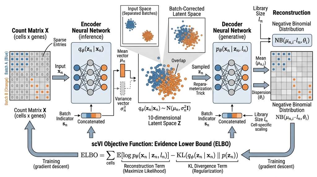
Figure 48.3 illustrates the scVI architecture. The encoder compresses each cell's gene expression vector and batch label into a low-dimensional latent code, while the decoder reconstructs the expected counts conditioned on both the latent code and the batch identity. This encoder-decoder structure ensures that the latent space captures biology, not batch artifacts. Figure 48.3.1 illustrates scVI variational autoencoder architecture for single-cell batch correction.

Mental Model

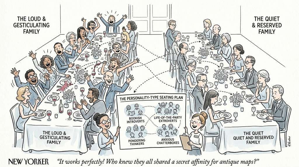
Think of scVI's latent space like a seating chart at a wedding with guests from two families (batches). Each guest (cell) has a personality profile (gene expression), but their behavior is also shaped by which family's table they sit at (batch effects): the loud family talks more, the quiet family less. scVI learns to separate personality from table assignment. The encoder strips away the table effect to find each guest's true personality (latent code), and the decoder can reconstruct how any guest would behave at any table. The ELBO training objective ensures the personality descriptions are compact (the KL term, like a word limit on the seating card) while still faithfully predicting behavior (the reconstruction term, like checking the card against actual conversations). The result is a personality map where similar people sit near each other regardless of which family they arrived with.

import scvi
import anndata as ad

def train_scvi(
    adata: ad.AnnData,
    batch_key: str = "batch",
    n_latent: int = 10,
    n_layers: int = 2,
    n_hidden: int = 128,
    max_epochs: int = 200,
) -> scvi.model.SCVI:
    """Train scVI for batch-corrected latent representation.

    The model learns a low-dimensional embedding that captures
    biological variation while removing batch-specific effects.

    Args:
        adata: AnnData with raw counts in adata.X or adata.layers["counts"]
        batch_key: column in adata.obs identifying batches
        n_latent: dimensionality of the latent space
        n_layers: number of hidden layers in encoder/decoder
        n_hidden: hidden layer width

    Returns: trained scVI model
    """
    # Register the AnnData object with scVI
    scvi.model.SCVI.setup_anndata(
        adata,
        layer="counts" if "counts" in adata.layers else None,
        batch_key=batch_key,
    )

    # Create and train the model
    model = scvi.model.SCVI(
        adata,
        n_latent=n_latent,
        n_layers=n_layers,
        n_hidden=n_hidden,
        gene_likelihood="nb",  # Negative binomial
    )

    model.train(
        max_epochs=max_epochs,
        early_stopping=True,
        early_stopping_patience=10,
    )

    return model


def get_latent_representation(model: scvi.model.SCVI, adata: ad.AnnData):
    """Extract batch-corrected latent representation.

    The latent space captures biological variation with batch
    effects removed. Use for clustering, visualization, and
    differential expression.
    """
    # Get latent representation (batch-corrected)
    latent = model.get_latent_representation()
    adata.obsm["X_scVI"] = latent

    # Compute neighbors and UMAP in the scVI latent space
    import scanpy as sc
    sc.pp.neighbors(adata, use_rep="X_scVI")
    sc.tl.umap(adata)
    sc.tl.leiden(adata, resolution=0.8)  # Leiden: a graph-based community detection algorithm that partitions cells into clusters

    return adata


def differential_expression(
    model: scvi.model.SCVI,
    adata: ad.AnnData,
    group1: str,
    group2: str,
    groupby: str = "leiden",
) -> "pd.DataFrame":
    """Bayesian differential expression between cell groups.

    scVI's DE test uses the generative model to compute
    posterior log-fold changes and Bayes factors (the ratio of
    evidence for differential expression versus no change),
    avoiding the distributional assumptions of t-tests or
    Wilcoxon tests.
    """
    de_results = model.differential_expression(
        adata,
        groupby=groupby,
        group1=group1,
        group2=group2,
    )

    # Filter significant genes
    significant = de_results[
        (de_results["is_de_fdr_0.05"]) &
        (abs(de_results["lfc_mean"]) > 0.5)
    ]

    return significant.sort_values("lfc_mean", ascending=False)

Once scVI produces a batch-corrected latent space, the natural next question is whether those embeddings can also assign biological identities to cells, particularly when only a fraction of cells carry expert-curated labels.

3. scANVI: Semi-Supervised Cell Annotation

scANVI extends scVI with a semi-supervised classification layer. Given a dataset where some cells have known type labels and others do not, scANVI simultaneously learns the latent representation and transfers labels to unlabeled cells. The generative model adds a discrete cell-type variable \(c_n\):

For labeled cells, \(c_n\) is observed; for unlabeled cells, it is treated as a latent variable and marginalized (summed over all possible cell-type values so the model considers every assignment weighted by its probability). The classifier \(q_\phi(c_n | \mathbf{z}_n)\) learns to predict cell types from the latent representation, enabling label transfer across datasets, batches, and even species.

def train_scanvi(
    adata: ad.AnnData,
    labels_key: str = "cell_type",
    unlabeled_category: str = "Unknown",
    batch_key: str = "batch",
    n_latent: int = 10,
) -> scvi.model.SCANVI:
    """Train scANVI for semi-supervised cell type annotation.

    Uses labeled cells to learn a classifier that transfers
    annotations to unlabeled cells, even across batches.
    """
    # First train scVI as initialization
    scvi.model.SCVI.setup_anndata(
        adata, batch_key=batch_key,
        layer="counts" if "counts" in adata.layers else None,
    )
    scvi_model = scvi.model.SCVI(adata, n_latent=n_latent)
    scvi_model.train(max_epochs=100, early_stopping=True)

    # Initialize scANVI from pretrained scVI
    scanvi_model = scvi.model.SCANVI.from_scvi_model(
        scvi_model,
        adata=adata,
        labels_key=labels_key,
        unlabeled_category=unlabeled_category,
    )

    scanvi_model.train(max_epochs=50, early_stopping=True)

    # Predict labels for unlabeled cells
    predictions = scanvi_model.predict()
    adata.obs["predicted_cell_type"] = predictions

    return scanvi_model

4. scGPT: A Foundation Model for Single-Cell Biology

scGPT applies the transformer pretraining paradigm to single-cell transcriptomics. The model treats each cell's gene expression profile as a "sentence" where genes are "tokens" and expression levels are "values." Pretraining uses a masked gene expression prediction objective: given a subset of a cell's gene expression values, predict the masked genes.

The input representation has three components per gene:

• Gene token embedding: a learned vector for each gene identity.
• Expression value embedding: the log-normalized expression value, binned into discrete levels and embedded.
• Condition embedding: optional metadata (batch, perturbation, cell type) encoded as additional tokens.

The model is pretrained on 33 million cells from the CELLxGENE database (circa 2023), learning representations that transfer to downstream tasks. (After pretraining on those 33 million unlabeled cells, scGPT reaches 85 to 95% annotation accuracy on published benchmarks with only a few hundred labeled examples per cell type, a ratio of roughly 100,000 unlabeled cells per labeled one.) (as of 2025, newer single-cell foundation models such as scGPT-2 and scFoundation have scaled pretraining to over 50 million cells with improved architectures, though the original scGPT remains widely used as a baseline):

import scgpt
from scgpt.model import TransformerModel
from scgpt.tokenizer import GeneVocab
from scgpt.utils import set_seed
import torch

def finetune_scgpt_for_annotation(
    adata_train: "ad.AnnData",
    adata_test: "ad.AnnData",
    pretrained_model_dir: str,
    cell_type_key: str = "cell_type",
    max_epochs: int = 30,
    batch_size: int = 64,
    learning_rate: float = 1e-4,
) -> dict:
    """Fine-tune scGPT for cell type annotation.

    Uses a pretrained scGPT model and fine-tunes the
    classification head on a labeled training set.

    The pretrained model captures general cellular biology;
    fine-tuning adapts it to a specific tissue or disease context.
    """
    set_seed(42)

    # Load pretrained model and vocabulary
    vocab = GeneVocab.from_file(f"{pretrained_model_dir}/vocab.json")
    model_config = scgpt.load_config(f"{pretrained_model_dir}/config.json")

    model = TransformerModel(
        ntoken=len(vocab),
        d_model=model_config["embsize"],
        nhead=model_config["nheads"],
        d_hid=model_config["d_hid"],
        nlayers=model_config["nlayers"],
        nlayers_cls=3,  # Classification head layers
        n_cls=len(adata_train.obs[cell_type_key].unique()),
        vocab=vocab,
    )

    # Load pretrained weights
    model.load_pretrained(f"{pretrained_model_dir}/best_model.pt")
    model = model.cuda()

    # Prepare data loaders
    from scgpt.data import prepare_dataloader
    train_loader = prepare_dataloader(
        adata_train, vocab, batch_size=batch_size,
        cell_type_key=cell_type_key, shuffle=True,
    )
    test_loader = prepare_dataloader(
        adata_test, vocab, batch_size=batch_size,
        cell_type_key=cell_type_key, shuffle=False,
    )

    # Fine-tune with classification loss
    optimizer = torch.optim.AdamW(model.parameters(), lr=learning_rate)
    criterion = torch.nn.CrossEntropyLoss()

    best_accuracy = 0.0
    for epoch in range(max_epochs):
        model.train()
        total_loss = 0.0
        for batch in train_loader:
            optimizer.zero_grad()
            output = model(batch["gene_ids"].cuda(), batch["values"].cuda())
            loss = criterion(output["cls_output"], batch["labels"].cuda())
            loss.backward()
            optimizer.step()
            total_loss += loss.item()

        # Evaluate
        model.eval()
        correct, total = 0, 0
        with torch.no_grad():
            for batch in test_loader:
                output = model(batch["gene_ids"].cuda(), batch["values"].cuda())
                preds = output["cls_output"].argmax(dim=1)
                correct += (preds == batch["labels"].cuda()).sum().item()
                total += len(preds)

        accuracy = correct / total
        best_accuracy = max(best_accuracy, accuracy)

    return {"best_accuracy": best_accuracy, "model": model}

5. Geneformer: Transfer Learning for Network Biology

Geneformer approaches single-cell foundation modeling differently: it rank-orders genes within each cell by expression level and processes the ranked list as a token sequence. This representation is inherently normalized, immune to library size variation, and encodes each gene's relative importance in the cell's regulatory program.

The model uses a standard transformer encoder pretrained with masked token prediction on approximately 30 million single-cell transcriptomes from the Genecorpus-30M dataset (Theodoris et al., Nature, 2023). The key applications are:

• Gene dosage sensitivity prediction: which genes, when their expression is halved (haploinsufficiency, the condition where a single functional copy of a gene is insufficient to maintain normal function), cause disease? Geneformer predicts this by measuring how much the model's attention patterns change when a gene is removed.
• In silico perturbation: predict the effect of knocking out or overexpressing a gene by modifying the input token sequence and observing changes in the model's output embedding.
• Chromatin dynamics: predict how gene regulatory states change during cell differentiation.

As of 2025, Geneformer 2 has expanded pretraining to over 95 million single-cell transcriptomes and added multi-task fine-tuning heads, improving performance on dosage sensitivity and perturbation response benchmarks compared to the original release. The rank-order tokenization strategy described here remains unchanged in the newer version.

from geneformer import InSilicoPerturber, EmbExtractor
from geneformer import TranscriptomeTokenizer

def run_in_silico_perturbation(
    model_dir: str,
    tokenized_dataset_path: str,
    genes_to_perturb: list[str],
    cell_type_col: str = "cell_type",
) -> dict:
    """Predict the effect of gene perturbations using Geneformer.

    Simulates gene knockouts by removing genes from the ranked
    expression list and measuring the shift in cell embeddings.

    A large embedding shift indicates the gene is important for
    maintaining the cell's identity/state.
    """
    # Extract baseline embeddings
    extractor = EmbExtractor(
        model_type="Pretrained",
        num_classes=0,
        emb_mode="cell",
        filter_data={cell_type_col: ["T cell", "B cell", "Monocyte"]},
        max_ncells=10000,
        emb_layer=-1,
    )

    baseline_embs = extractor.extract_embs(
        model_dir, tokenized_dataset_path, output_dir="./embeddings"
    )

    # Run in silico perturbation
    perturber = InSilicoPerturber(
        perturb_type="delete",  # Simulate knockout
        perturb_rank_shift=None,
        genes_to_perturb=genes_to_perturb,
        model_type="Pretrained",
        num_classes=0,
        emb_mode="cell",
        cell_states_to_model={
            cell_type_col: {
                "start": "T cell",
                "goal": "B cell",
                "alt": "Monocyte",
            }
        },
    )

    perturber.perturb_data(
        model_dir, tokenized_dataset_path, output_dir="./perturbations"
    )

    return {"status": "complete", "output_dir": "./perturbations"}

import scanpy as sc

adata = sc.read_h5ad("pbmc_10k.h5ad")
sc.pp.normalize_total(adata)
sc.pp.log1p(adata)
sc.pp.highly_variable_genes(adata, n_top_genes=2000)
sc.pp.pca(adata)
sc.pp.neighbors(adata)
sc.tl.umap(adata)
sc.tl.leiden(adata, resolution=0.5)
sc.tl.rank_genes_groups(adata, "leiden", method="wilcoxon")
sc.pl.rank_genes_groups(adata, n_genes=10, save="markers.pdf")

Foundation models like scGPT and Geneformer learn rich representations of cellular state, but their most consequential use goes beyond classification: predicting what happens to a cell when you intervene on its genome.

6. Perturbation Prediction and Gene Regulatory Networks

Among the most consequential applications of single-cell foundation models is predicting the outcome of genetic perturbations before performing them. Perturb-seq experiments combine Clustered Regularly Interspaced Short Palindromic Repeats (CRISPR) gene knockouts with single-cell sequencing, measuring how each knockout changes the expression of all other genes. This produces a perturbation response matrix (a genes-by-knockouts table where each column records the expression changes caused by removing one gene) that captures causal regulatory relationships.

Foundation models trained on large Perturb-seq datasets can predict perturbation responses for unseen gene knockouts. The prediction problem: given a cell in state \(\mathbf{x}\) and a perturbation to gene \(g\), predict the post-perturbation expression state \(\mathbf{x}'\). This connects directly to the causal inference framework from Chapter 31. Each perturbation acts as an intervention, and the cell's response reveals causal structure in the gene regulatory network.

import numpy as np
from scipy.stats import pearsonr

def evaluate_perturbation_prediction(
    predicted: np.ndarray,
    observed: np.ndarray,
    control: np.ndarray,
    top_k: int = 50,
) -> dict:
    """Evaluate perturbation prediction quality.

    Metrics:
    - Pearson correlation on differentially expressed genes
    - Mean squared error on top-k affected genes
    - Direction accuracy (fraction of genes with correctly
      predicted up/down regulation)

    Args:
        predicted: predicted post-perturbation expression (n_genes,)
        observed: actual post-perturbation expression (n_genes,)
        control: unperturbed control expression (n_genes,)
    """
    # Compute fold changes
    pred_fc = predicted - control
    obs_fc = observed - control

    # Identify top-k most affected genes (by observed fold change)
    top_indices = np.argsort(np.abs(obs_fc))[-top_k:]

    # Pearson correlation on top-k genes
    r, p_value = pearsonr(pred_fc[top_indices], obs_fc[top_indices])

    # Mean squared error on top-k
    mse = np.mean((pred_fc[top_indices] - obs_fc[top_indices]) ** 2)

    # Direction accuracy
    pred_direction = np.sign(pred_fc[top_indices])
    obs_direction = np.sign(obs_fc[top_indices])
    direction_acc = np.mean(pred_direction == obs_direction)

    return {
        "pearson_r": float(r),
        "pearson_p": float(p_value),
        "mse_top_k": float(mse),
        "direction_accuracy": float(direction_acc),
    }

Beyond predicting individual perturbation outcomes, these models also enable inference of gene regulatory networks (GRNs): directed graphs where an edge from gene A to gene B means that changing A's expression causes a downstream change in B. By systematically predicting knockouts for every gene in a cell type and recording which other genes shift in response, researchers can reconstruct a full regulatory wiring diagram without performing every experiment in the lab. The resulting GRN complements the causal discovery methods from Chapter 31, grounding abstract causal graphs in measurable molecular mechanisms.

7. Discovery Workbench Integration

The Discovery Workbench gains a SingleCellAnalyzer component that wraps scVI for data integration, scANVI for annotation, and the perturbation prediction pipeline. Users provide AnnData objects from multiple experiments, and the component produces batch-corrected embeddings, cell-type annotations, and differential expression results, with all parameters and results logged to the experiment registry.

from discovery_workbench import Analyzer, ExperimentRegistry

class SingleCellAnalyzer(Analyzer):
    """Single-cell analysis pipeline for the Discovery Workbench."""

    def integrate_and_annotate(
        self,
        datasets: list["ad.AnnData"],
        reference_labels: str = "cell_type",
        batch_key: str = "dataset",
    ) -> "ad.AnnData":
        """Integrate multiple datasets with batch correction and annotation.

        Pipeline: concatenate -> scVI integration -> scANVI annotation
        """
        import anndata as ad

        # Concatenate datasets with batch labels
        combined = ad.concat(datasets, label=batch_key)
        self.registry.log("input", {
            "n_datasets": len(datasets),
            "total_cells": combined.n_obs,
        })

        # Train scVI for integration
        scvi_model = train_scvi(combined, batch_key=batch_key)
        combined = get_latent_representation(scvi_model, combined)

        # Train scANVI for annotation transfer
        scanvi_model = train_scanvi(
            combined, labels_key=reference_labels, batch_key=batch_key
        )

        self.registry.log("integration", {
            "n_clusters": len(combined.obs["leiden"].unique()),
            "annotation_accuracy": scanvi_model.history["accuracy"][-1],
        })

        return combined