34.1 Generative Models as Hypothesis Generators

1. The Generative Modeling Problem

Traditional screening libraries contain millions of compounds, yet cover less than 0.001% of estimated drug-like chemical space; when a promising target has no known binders, exhaustive search is simply futile. Generative models bypass that bottleneck by learning to propose candidates directly from the highest-probability regions of chemical space. What if you could hand a machine the entire known pharmacopeia and ask it to invent the next antibiotic? Given a dataset \(\mathcal{D} = \{x_1, x_2, \ldots, x_N\}\) drawn from an unknown data distribution \(p_{\text{data}}(x)\), a generative model learns an approximation \(p_\theta(x)\) from which we can sample new data points. In scientific contexts, \(x\) might represent a molecular graph, a protein backbone, a crystal structure, or a material composition. The quality of the generative model depends on two properties: coverage (can it generate all valid structures in the target distribution?) and precision (does every generated sample satisfy the validity constraints of the domain?).

A generative model defines a parametric probability distribution \(p_\theta(x)\) fitted to observed data. New samples drawn from \(p_\theta\) should be statistically indistinguishable from samples drawn from the true data distribution \(p_{\text{data}}\). The model proposes candidates that have never been observed, rather than analyzing existing data. That proposal loop is the core of scientific hypothesis generation. The mechanism is density estimation: the model learns where probability mass concentrates in data space. For example, it identifies which regions of chemical space contain drug-like molecules. Sampling from that learned density produces new points in high-probability regions. Use a generative model instead of a discriminative one whenever the goal is to propose new candidates rather than classify existing ones. Use retrieval or combinatorial enumeration when the search space is small enough to enumerate explicitly (fewer than roughly \(10^6\) candidates).

Coverage and precision define the core discovery trade-off. High coverage with low precision produces many invalid molecules alongside a few interesting ones. High precision with low coverage yields valid but unoriginal molecules from a narrow region of chemical space. Each generative architecture balances this trade-off differently. In short: A generative model is a machine for proposing what has never been observed, and the art lies in ensuring those proposals are not just novel but physically real.

In practice, generative models serve as hypothesis generators through a propose-evaluate-refine cycle. The model proposes candidate structures (molecules, proteins, materials) by sampling from its learned distribution. A domain-specific evaluator (a docking simulation, a property predictor, a physics-based energy function) scores each candidate. The scores then feed back into the model, either by retraining on the highest-scoring candidates, by adjusting the sampling distribution through conditioning, or by optimizing directly in the latent space. Each iteration narrows the search toward structures that are both statistically plausible and scientifically useful. The architectures surveyed below differ in how they represent the learned distribution and how readily they support this feedback loop.

2. Variational Autoencoders (VAEs)

A variational autoencoder (Kingma and Welling, 2014) introduces a latent variable \(z\) and factorizes generation into two steps: sample \(z \sim p(z)\) from a simple prior (usually a standard normal), then map \(z\) to data space with a decoder \(p_\theta(x|z)\). The marginal likelihood of the data is:

This integral is intractable for nonlinear decoders. The VAE sidesteps this by introducing an encoder \(q_\phi(z|x)\) that approximates the true posterior \(p_\theta(z|x)\), then optimizing the Evidence Lower BOund (ELBO):

The first term is the reconstruction loss: the decoder must reconstruct the input from the latent code. The second term is the Kullback-Leibler (KL) regularization: the encoder's posterior should stay close to the prior. This creates a tension. Strong regularization (\(D_{\text{KL}} \to 0\)) makes the latent space smooth and interpolable but degrades reconstruction. Weak regularization gives sharp reconstructions but a disorganized latent space where sampling from the prior produces garbage.

The reparameterization trick makes the ELBO differentiable with respect to \(\phi\). Instead of sampling \(z \sim q_\phi(z|x) = \mathcal{N}(\mu_\phi(x), \sigma_\phi^2(x))\) directly (which blocks gradient flow), we write \(z = \mu_\phi(x) + \sigma_\phi(x) \cdot \epsilon\) where \(\epsilon \sim \mathcal{N}(0, I)\). The randomness is now in \(\epsilon\), independent of \(\phi\), so gradients pass through \(\mu_\phi\) and \(\sigma_\phi\) normally.

import torch
import torch.nn as nn
import torch.nn.functional as F

class MolecularVAE(nn.Module):
    """VAE for SMILES-encoded molecules."""

    def __init__(self, vocab_size: int, max_len: int, latent_dim: int = 128):
        super().__init__()
        self.max_len = max_len
        self.latent_dim = latent_dim

        # Encoder: 1D convolutions over SMILES characters
        self.conv1 = nn.Conv1d(vocab_size, 64, kernel_size=9, padding=4)
        self.conv2 = nn.Conv1d(64, 64, kernel_size=9, padding=4)
        self.conv3 = nn.Conv1d(64, 32, kernel_size=11, padding=5)
        self.fc_enc = nn.Linear(32 * max_len, 256)
        self.fc_mu = nn.Linear(256, latent_dim)
        self.fc_logvar = nn.Linear(256, latent_dim)

        # Decoder: GRU over latent code
        self.fc_dec = nn.Linear(latent_dim, 256)
        self.gru = nn.GRU(256, 512, num_layers=3, batch_first=True)
        self.fc_out = nn.Linear(512, vocab_size)

    def encode(self, x):
        """x: (batch, vocab_size, max_len) one-hot encoded SMILES."""
        h = F.relu(self.conv1(x))
        h = F.relu(self.conv2(h))
        h = F.relu(self.conv3(h))
        h = h.view(h.size(0), -1)
        h = F.relu(self.fc_enc(h))
        return self.fc_mu(h), self.fc_logvar(h)

    def reparameterize(self, mu, logvar):
        """Sample z = mu + sigma * epsilon (reparameterization trick)."""
        std = torch.exp(0.5 * logvar)
        eps = torch.randn_like(std)
        return mu + std * eps

    def decode(self, z):
        """z: (batch, latent_dim) -> (batch, max_len, vocab_size) logits."""
        h = F.relu(self.fc_dec(z))
        h = h.unsqueeze(1).repeat(1, self.max_len, 1)  # repeat for each position
        h, _ = self.gru(h)
        return self.fc_out(h)

    def forward(self, x):
        mu, logvar = self.encode(x)
        z = self.reparameterize(mu, logvar)
        recon = self.decode(z)
        return recon, mu, logvar

def vae_loss(recon_logits, target, mu, logvar):
    """ELBO loss: reconstruction (cross-entropy) + KL divergence."""
    # Reconstruction: cross-entropy per character position
    recon_loss = F.cross_entropy(
        recon_logits.view(-1, recon_logits.size(-1)),
        target.view(-1),
        reduction='mean'
    )
    # KL divergence: closed form for diagonal Gaussian vs N(0,I)
    kl_loss = -0.5 * torch.mean(1 + logvar - mu.pow(2) - logvar.exp())
    return recon_loss + kl_loss

Molecular VAEs typically achieve roughly 70 to 85% validity (fraction of generated SMILES that parse into valid molecules) on drug-like compound datasets, depending on architecture and hyperparameter choices. The primary failure mode is the KL-reconstruction trade-off: the model either memorizes training molecules (low KL) or generates diverse but often invalid structures (high KL). The \(\beta\)-VAE variant (Higgins et al., 2017) adds a weight \(\beta\) to the KL term, letting you tune this trade-off explicitly.

3. Generative Adversarial Networks (GANs)

The VAE's explicit density model and smooth latent space come at the cost of blurry outputs; GANs sacrifice those properties in favor of sharp, high-fidelity samples by eliminating the likelihood function entirely.

GANs (Goodfellow et al., 2014) take a completely different approach: train a generator \(G_\theta\) to map noise \(z \sim p(z)\) to data space, while simultaneously training a discriminator \(D_\phi\) to distinguish real data from generated samples. The two networks play a minimax game:

At equilibrium (if it exists), the generator produces samples indistinguishable from real data. The theoretical appeal is that GANs do not require an explicit likelihood function, making them applicable to complex data types where defining \(p_\theta(x)\) is difficult. Unlike VAEs, which optimize a bound on the log-likelihood, GANs learn through a game between two networks, so their quality signal comes from the discriminator rather than from an explicit probability computation.

In practice, GANs for scientific applications, particularly drug discovery, face two serious problems. Mode collapse, where the generator learns to produce a small set of high-quality samples that fool the discriminator, ignoring most of the data distribution: for drug discovery, this means the model might generate 50 variants of aspirin and nothing else. Training instability: the generator and discriminator can oscillate rather than converge, requiring careful hyperparameter tuning and architectural choices. The Wasserstein GAN (Arjovsky et al., 2017) partially addresses both problems. It replaces the Jensen-Shannon divergence (a symmetric measure of how different two probability distributions are, derived from KL divergence) with the Wasserstein distance (also called earth mover's distance, a measure of the minimum "work" needed to transform one probability distribution into another) , providing smoother gradients. The Wasserstein distance also yields a meaningful training signal even when the generator distribution does not overlap with the data distribution.

4. Autoregressive Models and Normalizing Flows

Autoregressive models factorize the joint distribution as a product of conditionals:

Each token (atom, bond, or SMILES character) is generated conditioned on all previous tokens. This is the architecture behind language models, and it transfers naturally to molecular strings. The advantage is exact likelihood computation and stable training. The disadvantage for 3D scientific structures is that the sequential generation order is arbitrary: there is no natural "first atom" in a molecule. Graph-based autoregressive models (You et al., 2018) generate molecules node by node, choosing which atom to add next and where to connect it. These achieve higher validity (often 95%+) than SMILES-based models because each step can check chemical valency constraints before committing. (That gap matters: a SMILES-based VAE producing 70% valid molecules wastes nearly a third of every generation batch, while a graph-based autoregressive model at 95%+ validity makes almost every sample usable.)

Normalizing flows (Rezende and Mohamed, 2015) construct an invertible mapping \(f_\theta: \mathbb{R}^d \to \mathbb{R}^d\) that transforms a simple base distribution (Gaussian) into the data distribution. The change-of-variables formula gives the exact log-likelihood:

where the determinant of the Jacobian \(\frac{\partial f_\theta^{-1}}{\partial x}\) accounts for how the transformation stretches or compresses volume in data space (intuitively, regions where the mapping compresses many data points into a small latent region receive higher density). Flows provide exact likelihood and exact sampling (both forward and inverse passes are available), making them attractive for density estimation. However, the invertibility constraint limits architectural expressiveness. Continuous normalizing flows (CNFs), which parameterize the transformation as an ODE, relax this constraint at the cost of requiring an ODE solver during training. Flow matching (Section 34.2) builds on this idea while avoiding the ODE solver bottleneck.

import torch
import torch.nn as nn
from torch.distributions import Normal

class AffineCouplingLayer(nn.Module):
    """Single affine coupling layer for a normalizing flow."""

    def __init__(self, dim: int, hidden_dim: int = 256):
        super().__init__()
        half = dim // 2
        # Scale and translation networks
        self.scale_net = nn.Sequential(
            nn.Linear(half, hidden_dim), nn.ReLU(),
            nn.Linear(hidden_dim, hidden_dim), nn.ReLU(),
            nn.Linear(hidden_dim, dim - half), nn.Tanh()
        )
        self.translate_net = nn.Sequential(
            nn.Linear(half, hidden_dim), nn.ReLU(),
            nn.Linear(hidden_dim, hidden_dim), nn.ReLU(),
            nn.Linear(hidden_dim, dim - half)
        )

    def forward(self, x):
        """Forward pass: data -> latent (used for training)."""
        x1, x2 = x.chunk(2, dim=-1)
        s = self.scale_net(x1)       # log-scale
        t = self.translate_net(x1)   # translation
        y2 = x2 * torch.exp(s) + t   # affine transform
        log_det = s.sum(dim=-1)       # log determinant of Jacobian
        return torch.cat([x1, y2], dim=-1), log_det

    def inverse(self, y):
        """Inverse pass: latent -> data (used for sampling)."""
        y1, y2 = y.chunk(2, dim=-1)
        s = self.scale_net(y1)
        t = self.translate_net(y1)
        x2 = (y2 - t) * torch.exp(-s)
        return torch.cat([y1, x2], dim=-1)

class NormalizingFlow(nn.Module):
    """Stack of affine coupling layers with permutations."""

    def __init__(self, dim: int, n_layers: int = 6, hidden_dim: int = 256):
        super().__init__()
        self.layers = nn.ModuleList([
            AffineCouplingLayer(dim, hidden_dim) for _ in range(n_layers)
        ])
        self.base_dist = Normal(torch.zeros(dim), torch.ones(dim))
        # Alternating permutation indices
        self.perms = [torch.randperm(dim) for _ in range(n_layers)]

    def log_prob(self, x):
        """Compute exact log-likelihood via change of variables."""
        log_det_total = 0
        z = x
        for layer, perm in zip(self.layers, self.perms):
            z = z[:, perm]  # permute dimensions
            z, log_det = layer(z)
            log_det_total += log_det
        log_pz = self.base_dist.log_prob(z).sum(dim=-1)
        return log_pz + log_det_total

    def sample(self, n: int):
        """Generate samples by inverting the flow."""
        z = self.base_dist.sample((n,))
        x = z
        for layer, perm in zip(reversed(self.layers), reversed(self.perms)):
            x = layer.inverse(x)
            inv_perm = torch.argsort(perm)
            x = x[:, inv_perm]
        return x

5. Why Diffusion Models Won

Each of the architectures above offers a distinct mathematical trade-off, yet all share a common vulnerability: at least one failure mode (mode collapse, KL-reconstruction tension, invertibility constraints) that limits reliability in scientific applications.

By 2022, diffusion models had largely displaced VAEs, GANs, and flows as the dominant architecture for both image generation and scientific applications. Four properties account for this shift.

Training stability. Diffusion models optimize a simple denoising objective: predict the noise added to a data point. There is no adversarial game (GANs), no KL-reconstruction trade-off (VAEs), and no architectural constraint (flows). The loss landscape is smooth, and training reliably converges without extensive hyperparameter tuning.

Mode coverage. Because diffusion models are trained to denoise from every noise level, they see the full data distribution at every training step. This largely eliminates the mode collapse problem that plagues GANs. In molecular generation, coverage translates directly to chemical diversity: the model explores the full space of valid structures rather than memorizing a subset.

Beyond Sample Quality

Conditioning flexibility. Adding conditional information (target protein structure, desired molecular properties, binding pocket geometry) is straightforward: classifier-free guidance, where the model learns both conditional and unconditional generation and interpolates between them at inference time , provides a general mechanism that works with any conditioning signal without architectural changes. Section 34.4 covers this in depth.

Compositionality. Diffusion models naturally compose: you can combine multiple guidance signals (bind this target AND be synthesizable AND have low toxicity) at inference time without retraining. For discovery, where the objective is always multi-dimensional, this is crucial.

6. The Generative Landscape for Discovery

Diffusion models may dominate, but they did not eliminate the earlier architectures; each retains a niche where its particular strengths still matter.

Each architecture occupies a niche in the current discovery landscape, as summarized in Figure 34.1. VAEs remain useful when you need a smooth, interpretable latent space for optimization (navigating chemical space by interpolating latent codes). GANs persist in applications where sample quality matters more than diversity (generating high-resolution microscopy images for data augmentation). Autoregressive models dominate protein sequence generation (as in Evolutionary Scale Modeling (ESM) based design; as of 2024, ESM3, a multimodal generative model over sequence, structure, and function, has extended this family beyond pure autoregression) because the sequential nature of amino acid chains maps naturally to left-to-right generation. Normalizing flows appear in Boltzmann generators, where Boltzmann generators are normalizing flows trained to sample from a physical system's Boltzmann distribution so that exact likelihood enables computation of thermodynamic quantities like free energy differences (see Chapter 43: Scientific Simulation). Figure 34.1.1 illustrates Generative architecture comparison: VAE, GAN, Autoregressive, Normalizing Flow, and Diffusion.

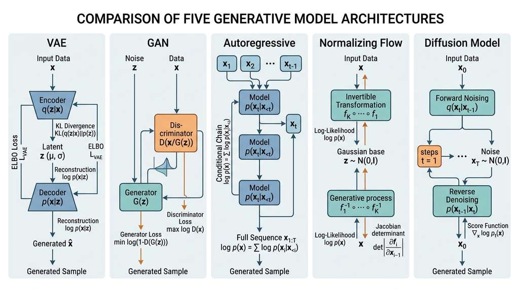
Diffusion models and their close relative, flow matching, dominate 3D structure generation: molecules, proteins, crystals, and materials. Their combination of training stability, mode coverage, and conditioning flexibility makes them the default choice for de novo design. The next three sections focus on this dominant paradigm: Section 34.2 covers the mathematical foundations of score-based diffusion and flow matching; Section 34.3 extends these ideas to equivariant generation on 3D structures; and Section 34.4 addresses conditioning, optimization, and evaluation.

Exercises

1. (Conceptual) Explain why mode collapse in a GAN is particularly harmful for drug discovery compared to image generation. What scientific consequence would it have if your molecular generator only produced variations of a few scaffolds?
2. (Coding) Implement a \(\beta\)-VAE for molecular fingerprints (2048-dimensional binary vectors from RDKit Morgan fingerprints, where Morgan fingerprints are circular substructure hashes that encode the presence of molecular neighborhoods within a fixed radius around each atom ). Train on 10,000 molecules from the ZINC dataset. Vary \(\beta \in \{0.1, 0.5, 1.0, 5.0\}\) and measure reconstruction accuracy (Tanimoto similarity, where Tanimoto similarity is the ratio of shared bits to total set bits between two binary fingerprints , between input and reconstructed fingerprints) and latent space smoothness (average distance between interpolated decodings of neighboring molecules). Plot the trade-off curve.
3. (Analysis) Compare the sample quality (validity, uniqueness, novelty as defined in Section 34.4) of a SMILES-based autoregressive model versus a graph-based autoregressive model (GraphAF from TorchDrug) on the ZINC 250K subset. Which achieves higher validity? Explain the result in terms of the structural constraints each representation enforces during generation.