Bringing a drug from initial concept to approved therapy takes 10 to 15 years and costs over \$2.6 billion on average (circa 2020 Tufts CSDD estimate), with a 90% failure rate in clinical trials. AI cannot eliminate this uncertainty, but it can compress the early stages dramatically: identifying disease-relevant targets from genomic data, screening millions of candidate molecules computationally rather than physically, and predicting pharmacokinetic properties before synthesis. This section maps the drug discovery pipeline and shows exactly where AI methods slot in, what they accelerate, and what remains stubbornly resistant to computational shortcuts.
1. The Drug Discovery Pipeline
Every year, pharmaceutical companies abandon late-stage drug candidates after investing hundreds of millions of dollars, often because a flaw that was detectable at the screening stage slipped through unnoticed. Understanding exactly where candidates fail, and why, is the prerequisite for building AI systems that catch those flaws early.
Of the roughly 1060 drug-like molecules that are theoretically possible, fewer than 104 have ever reached a pharmacy shelf, and each of those survivors navigated a gauntlet that discards 99.9% of candidates at every stage. Understanding this pipeline is essential before applying AI to any part of it, because the value of a computational prediction depends entirely on where in the pipeline it sits.
The pipeline has five major stages:
- Target identification: finding the biological molecule (usually a protein) whose modulation will treat the disease.
- Hit finding: discovering chemical matter that interacts with the target, typically through high-throughput screening (HTS) or virtual screening.
- Lead optimization: iteratively modifying hits to improve potency, selectivity, and drug-like properties.
- Preclinical development: evaluating toxicity, pharmacokinetics, and formulation in animal models.
- Clinical trials: testing safety (Phase I), efficacy (Phase II), and comparative effectiveness (Phase III) in humans.
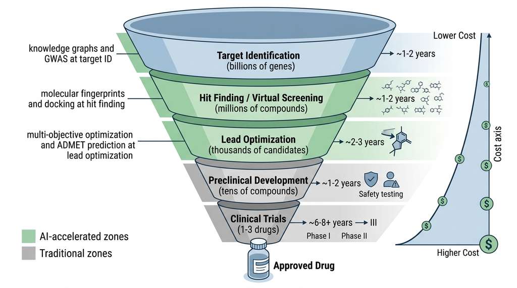
Figure 48.1 maps these five stages as a narrowing funnel, highlighting where AI methods currently deliver the greatest acceleration. Figure 48.1.1 illustrates Drug discovery pipeline funnel with AI intervention points.
AI has its greatest current impact in stages 1 through 3. Preclinical and clinical stages involve regulatory constraints, biological variability, and ethical considerations that limit purely computational approaches (though clinical AI, covered in Section 48.4, addresses trial design and patient stratification). In short: AI's highest leverage is at the cheapest, most uncertain end of the funnel, where a better computational filter today prevents a billion-dollar clinical failure years from now.
The drug discovery pipeline is a funnel with a paradoxical property: the cheapest stages (target ID, virtual screening) have the highest uncertainty, while the most expensive stages (clinical trials) have the lowest. AI's leverage comes from improving the quality of decisions at the cheap end, so fewer expensive failures occur downstream. A 10% improvement in hit quality can save hundreds of millions in late-stage attrition.
2. Target Identification with Genomics and Knowledge Graphs
Target identification asks: which protein, when inhibited or activated, will alter the disease phenotype? Traditional approaches relied on phenotypic screens (assays that measure a compound's effect on cells or organisms without knowing the molecular target) and literature curation. Modern AI-driven target ID combines three data sources: genome-wide association studies (GWAS), transcriptomic differential expression, and biomedical knowledge graphs.
Knowledge graphs for target identification connect genes, diseases, pathways, drugs, and side effects in a heterogeneous graph. Link prediction on this graph identifies gene-disease associations not yet reported in the literature. The approach from Chapter 38 applies directly. Train a graph embedding model (TransE, RotatE, or a GNN (graph neural network)-based encoder) on known associations, then rank candidate gene-disease links by predicted score.
import numpy as np
from pykeen.pipeline import pipeline
from pykeen.triples import TriplesFactory

def train_target_identification_model(
    triples_path: str,
    embedding_dim: int = 256,
    num_epochs: int = 200,
):
    """Train a knowledge graph embedding model for target identification.

    The triples file contains (gene, relation, disease) tuples from
    curated databases like DisGeNET, OMIM, and DrugBank.
    """
    tf = TriplesFactory.from_path(triples_path)
    training, testing, validation = tf.split([0.8, 0.1, 0.1])

    result = pipeline(
        training=training,
        testing=testing,
        validation=validation,
        model="RotatE",
        model_kwargs={"embedding_dim": embedding_dim},
        optimizer="Adam",
        optimizer_kwargs={"lr": 1e-3},
        training_kwargs={
            "num_epochs": num_epochs,
            "batch_size": 1024,
        },
        evaluation_kwargs={"batch_size": 256},
    )

    return result.model, result.metric_results


def predict_novel_targets(model, disease_entity: str, top_k: int = 50):
    """Predict novel gene targets for a disease.

    Returns genes ranked by predicted association score that are
    NOT in the training set (truly novel predictions).
    """
    predictions = model.predict_target(
        head=disease_entity,
        relation="associated_with",
    )
return predictions.topk(top_k)Mendelian randomization provides causal evidence for target-disease associations by using genetic variants as instrumental variables (factors that influence the outcome only through the gene of interest, creating a natural experiment). If a variant that reduces expression of gene \(G\) also reduces risk of disease \(D\), this constitutes causal evidence that inhibiting \(G\)'s protein product could treat \(D\). The causal inference methods from Chapter 31 formalize this reasoning.
3. Hit Finding: Virtual Screening
Once a target protein is identified, the next step is finding molecules that bind to it. Physical high-throughput screening tests hundreds of thousands of compounds in robotic assays. Virtual screening replaces physical testing with computational prediction, enabling screening of billions of molecules. (In reported prospective studies, AI-guided virtual screening has typically achieved hit rates of 10 to 12%, compared to roughly 0.1% from random physical screening: a 100x enrichment that turns a needle-in-a-haystack search into a targeted retrieval.)
Virtual screening evaluates large chemical libraries computationally to identify molecules likely to bind a biological target. No compound is synthesized or physically tested at this stage. Physical screening of even a million compounds costs millions of dollars and weeks of robotic assay time. Virtual screening evaluates billions of candidates on a GPU cluster in hours for a fraction of that cost. The process has two stages. First, each candidate molecule is represented numerically (as a fingerprint, a graph, or a 3D coordinate set). Then a scoring function ranks molecules by predicted binding strength or structural similarity to known actives. Use virtual screening when a validated target structure or known active ligands exist; when neither is available, phenotypic screening or fragment-based approaches remain necessary starting points.
Two complementary approaches dominate virtual screening:
3.1 Ligand-Based Virtual Screening
When known active molecules exist, ligand-based methods search for similar compounds. The key representation is the molecular fingerprint: a fixed-length binary or count vector encoding the presence of chemical substructures. Each molecule is specified as a SMILES (Simplified Molecular-Input Line-Entry System) string, a compact text notation where atoms are letters and bonds are symbols. RDKit provides several fingerprint types; the Morgan (circular) fingerprint with radius 2 is the most widely used:
from rdkit import Chem
from rdkit.Chem import AllChem, DataStructs
import numpy as np

def compute_morgan_fingerprint(smiles: str, radius: int = 2, n_bits: int = 2048):
    """Compute Morgan circular fingerprint from SMILES string.

    The Morgan fingerprint encodes circular substructures up to
    the specified radius. Each atom's neighborhood is hashed to
    a bit position, creating a fixed-length representation of
    the molecule's local chemical environments.
    """
    mol = Chem.MolFromSmiles(smiles)
    if mol is None:
        raise ValueError(f"Invalid SMILES: {smiles}")
    fp = AllChem.GetMorganFingerprintAsBitVect(mol, radius, nBits=n_bits)
    return np.array(fp)


def tanimoto_similarity(fp1: np.ndarray, fp2: np.ndarray) -> float:
    """Tanimoto coefficient between two binary fingerprints.

    T(A, B) = |A ∩ B| / |A ∪ B|

    Values above 0.4 indicate meaningful structural similarity.
    Values above 0.7 suggest similar biological activity.
    """
    intersection = np.sum(fp1 & fp2)
    union = np.sum(fp1 | fp2)
    if union == 0:
        return 0.0
    return intersection / union


def virtual_screen_ligand_based(
    query_smiles: str,
    library_smiles: list[str],
    threshold: float = 0.4,
) -> list[tuple[str, float]]:
    """Screen a compound library by similarity to a query molecule.

    Returns compounds with Tanimoto similarity above threshold,
    sorted by decreasing similarity.
    """
    query_fp = compute_morgan_fingerprint(query_smiles)
    hits = []
    for smiles in library_smiles:
        try:
            lib_fp = compute_morgan_fingerprint(smiles)
            sim = tanimoto_similarity(query_fp, lib_fp)
            if sim >= threshold:
                hits.append((smiles, sim))
        except ValueError:
            continue
return sorted(hits, key=lambda x: x[1], reverse=True)The Tanimoto coefficient between two fingerprints \(A\) and \(B\) is defined as:
$$T(A, B) = \frac{|A \cap B|}{|A \cup B|} = \frac{\sum_i \min(a_i, b_i)}{\sum_i \max(a_i, b_i)}$$For binary fingerprints, this simplifies to the ratio of shared "on" bits to the total number of "on" bits in either fingerprint.
Mental Model
Think of molecular fingerprints and Tanimoto similarity like comparing two recipes by their ingredient lists. Each recipe (molecule) is reduced to a checklist of ingredients (chemical substructures): "contains garlic" = 1, "contains saffron" = 0. The Tanimoto score is the fraction of ingredients shared by both recipes out of all ingredients mentioned by either one. Two recipes that share 8 out of 10 total ingredients (Tanimoto = 0.8) will likely taste similar, just as two molecules sharing most substructures will likely bind similar targets. The key limitation maps too: recipes with the same ingredients in different proportions can taste very different, just as molecules with identical substructure fingerprints can have different 3D shapes and therefore different binding behavior.
3.2 Structure-Based Virtual Screening (Docking)
When the target protein's 3D structure is available (from X-ray crystallography, cryogenic electron microscopy (cryo-EM), or AlphaFold prediction), molecular docking predicts how a small molecule binds in the protein's active site. Docking scores approximate binding free energy:
$$\Delta G_{\text{bind}} \approx \Delta G_{\text{vdW}} + \Delta G_{\text{elec}} + \Delta G_{\text{hbond}} + \Delta G_{\text{desolv}} + \Delta G_{\text{tors}}$$where the terms capture van der Waals interactions, electrostatics, hydrogen bonds, desolvation penalties (the energy cost of stripping water molecules from both the ligand and the binding pocket before they can interact), and torsional strain. More negative scores indicate stronger predicted binding.
Common Misconception
A frequent misconception is that a low (highly negative) docking score means a molecule will be an effective drug. In reality, docking scores predict only one narrow property: how well a molecule's shape complements the target protein's binding pocket in a static snapshot. A molecule can achieve an excellent docking score yet fail as a drug because it is metabolically unstable (destroyed by liver enzymes within minutes), cannot cross cell membranes to reach its target, binds dozens of unintended proteins causing toxic side effects, or is simply impossible to synthesize. Docking is a filter for geometric compatibility, not a predictor of therapeutic success.
import subprocess
import os
from dataclasses import dataclass

@dataclass
class DockingResult:
    ligand_smiles: str
    score: float  # kcal/mol (more negative = better)
    pose_file: str

def dock_molecule(
    ligand_smiles: str,
    receptor_pdbqt: str,
    center: tuple[float, float, float],
    box_size: tuple[float, float, float] = (25.0, 25.0, 25.0),
    exhaustiveness: int = 32,
    work_dir: str = "/tmp/docking",
) -> DockingResult:
    """Dock a single molecule against a receptor using AutoDock Vina.

    The binding site is defined by a center coordinate and box size
    in Angstroms. Exhaustiveness controls search thoroughness.
    """
    os.makedirs(work_dir, exist_ok=True)

    # Convert SMILES to 3D structure and prepare for docking
    from rdkit import Chem
    from rdkit.Chem import AllChem
    mol = Chem.MolFromSmiles(ligand_smiles)
    mol = Chem.AddHs(mol)
    AllChem.EmbedMolecule(mol, randomSeed=42)
    AllChem.MMFFOptimizeMolecule(mol)

    ligand_sdf = os.path.join(work_dir, "ligand.sdf")
    Chem.MolToMolFile(mol, ligand_sdf)

    # Convert to PDBQT format (required by Vina)
    ligand_pdbqt = os.path.join(work_dir, "ligand.pdbqt")
    subprocess.run([
        "mk_prepare_ligand.py", "-i", ligand_sdf, "-o", ligand_pdbqt
    ], check=True)

    # Run Vina docking
    output_pdbqt = os.path.join(work_dir, "output.pdbqt")
    result = subprocess.run([
        "vina",
        "--receptor", receptor_pdbqt,
        "--ligand", ligand_pdbqt,
        "--center_x", str(center[0]),
        "--center_y", str(center[1]),
        "--center_z", str(center[2]),
        "--size_x", str(box_size[0]),
        "--size_y", str(box_size[1]),
        "--size_z", str(box_size[2]),
        "--exhaustiveness", str(exhaustiveness),
        "--out", output_pdbqt,
    ], capture_output=True, text=True, check=True)

    # Parse best score from Vina output
    best_score = _parse_vina_score(result.stdout)

    return DockingResult(
        ligand_smiles=ligand_smiles,
        score=best_score,
        pose_file=output_pdbqt,
    )


def _parse_vina_score(vina_output: str) -> float:
    """Extract the best binding affinity from Vina output."""
    for line in vina_output.split("\n"):
        if line.strip().startswith("1"):
            parts = line.split()
            return float(parts[1])
raise ValueError("Could not parse Vina output")In 2023, researchers at Recursion Pharmaceuticals screened 36 billion molecules against a kinase target using a combination of 2D fingerprint pre-filtering and 3D docking. The first pass used Tanimoto similarity against known actives to reduce 36 billion to 500 million candidates (a 72x reduction in under an hour on a GPU cluster). The second pass docked these 500 million in AutoDock-GPU, taking three days on 1,000 GPUs. The third pass clustered the top 100,000 by chemical scaffold to ensure diversity. From 36 billion initial molecules, 2,000 were purchased and tested; 250 showed activity below 10 micromolar, a 12.5% hit rate compared to the typical 0.1% from random HTS.
4. Lead Optimization
Screening billions of molecules to find thousands of hits solves only the first half of the problem; the harder challenge is transforming a weak, imperfect binder into a compound safe and potent enough to enter a patient.
Lead optimization iterates on a hit's chemical structure to improve potency (binding affinity), selectivity (avoiding off-target binding), and drug-likeness (oral bioavailability, metabolic stability, low toxicity). This multi-objective optimization problem maps directly to the methods from Chapter 45.
4.1 ADMET Prediction
ADMET stands for Absorption, Distribution, Metabolism, Excretion, and Toxicity. These pharmacokinetic properties determine whether a molecule that binds a target in a test tube will work as a drug in a human body. AI models predict ADMET properties from molecular structure, enabling computational triage before synthesis.
Checkpoint
So far: ADMET captures the five pharmacokinetic dimensions (Absorption, Distribution, Metabolism, Excretion, Toxicity) that determine whether a molecule effective in a test tube will also work inside a living body; AI models now predict these properties from molecular structure alone, enabling computational triage before any compound is synthesized.
from rdkit import Chem
from rdkit.Chem import Descriptors, Lipinski

@dataclass
class ADMETProfile:
    molecular_weight: float
    logp: float
    hbd: int   # hydrogen bond donors
    hba: int   # hydrogen bond acceptors
    tpsa: float  # topological polar surface area
    rotatable_bonds: int
    lipinski_violations: int
    drug_likeness_score: float

def compute_admet_profile(smiles: str) -> ADMETProfile:
    """Compute ADMET-relevant molecular descriptors.

    Combines Lipinski's Rule of Five with additional descriptors
    (TPSA, rotatable bonds) that predict oral absorption.
    """
    mol = Chem.MolFromSmiles(smiles)
    if mol is None:
        raise ValueError(f"Invalid SMILES: {smiles}")

    mw = Descriptors.MolWt(mol)
    logp = Descriptors.MolLogP(mol)
    hbd = Lipinski.NumHDonors(mol)
    hba = Lipinski.NumHAcceptors(mol)
    tpsa = Descriptors.TPSA(mol)
    rot_bonds = Lipinski.NumRotatableBonds(mol)

    # Count Lipinski violations
    violations = sum([
        mw > 500,
        logp > 5,
        hbd > 5,
        hba > 10,
    ])

    # Quantitative Estimate of Drug-likeness (QED)
    from rdkit.Chem.QED import qed
    qed_score = qed(mol)

    return ADMETProfile(
        molecular_weight=mw,
        logp=logp,
        hbd=hbd,
        hba=hba,
        tpsa=tpsa,
        rotatable_bonds=rot_bonds,
        lipinski_violations=violations,
        drug_likeness_score=qed_score,
)4.2 Multi-Objective Lead Optimization
Lead optimization requires balancing competing objectives. A molecule with nanomolar binding affinity is useless if it is metabolically unstable or toxic. We formalize this as a multi-objective optimization problem:
$$\max_{\mathbf{x} \in \mathcal{X}} \; \bigl( f_{\text{potency}}(\mathbf{x}), \; f_{\text{selectivity}}(\mathbf{x}), \; f_{\text{QED}}(\mathbf{x}) \bigr)$$subject to constraints on molecular weight, log P, and synthesizability score (a computed estimate of how difficult a molecule would be to manufacture in a chemistry lab, where lower scores indicate easier synthesis). The Pareto optimization framework from Section 45.2 identifies the set of non-dominated solutions: molecules where no single property can be improved without degrading another.
from rdkit.Chem import RDConfig
import os
import sys

# Multi-property optimization with molecular generation
def optimize_lead(
    seed_smiles: str,
    target_protein_pdbqt: str,
    binding_site_center: tuple[float, float, float],
    n_iterations: int = 50,
    population_size: int = 100,
) -> list[dict]:
    """Multi-objective lead optimization using genetic algorithm.

    Objectives:
    1. Maximize predicted binding affinity (docking score)
    2. Maximize drug-likeness (QED)
    3. Minimize synthetic accessibility (SA score)

    Uses matched molecular pair transformations to generate
    neighboring molecules from the seed compound.
    """
    from rdkit.Chem import AllChem, RDConfig
    from rdkit.Chem.SA_Score import sascorer

    seed_mol = Chem.MolFromSmiles(seed_smiles)
    population = [seed_smiles]

    # Generate initial population via random modifications
    for _ in range(population_size - 1):
        mutant = _random_molecular_mutation(seed_mol)
        if mutant is not None:
            population.append(Chem.MolToSmiles(mutant))

    pareto_front = []
    for iteration in range(n_iterations):
        # Evaluate all objectives
        scored = []
        for smi in population:
            try:
                profile = compute_admet_profile(smi)
                dock_result = dock_molecule(
                    smi, target_protein_pdbqt, binding_site_center
                )
                mol = Chem.MolFromSmiles(smi)
                sa_score = sascorer.calculateScore(mol)

                scored.append({
                    "smiles": smi,
                    "docking_score": dock_result.score,
                    "qed": profile.drug_likeness_score,
                    "sa_score": sa_score,
                })
            except Exception:
                continue

        # Non-dominated sorting (NSGA-II style, where NSGA-II is a
        # multi-objective genetic algorithm that ranks solutions by
        # Pareto dominance and crowding distance)
        pareto_front = _non_dominated_sort(scored)

        # Generate next population from Pareto-optimal parents
        population = _breed_next_generation(pareto_front, population_size)

return pareto_frontThe Therapeutics Data Commons provides standardized benchmarks and datasets for every stage of the drug discovery pipeline. Instead of curating your own ADMET datasets and splitting them for evaluation, TDC provides ready-to-use data loaders with standard train/validation/test splits:
from tdc.single_pred import ADME

# Load the Caco-2 permeability dataset (intestinal absorption)
data = ADME(name="Caco2_Wang")
split = data.get_split(method="scaffold")  # Scaffold-based split

train = split["train"]  # SMILES + permeability values
valid = split["valid"]
test = split["test"]

print(f"Train: {len(train)}, Valid: {len(valid)}, Test: {len(test)}")
# Train: 728, Valid: 91, Test: 91
TDC covers 66 datasets across 22 tasks (circa 2022; the collection has since grown) spanning target discovery, activity modeling, ADMET prediction, and drug-drug interaction. Using standard benchmarks rather than custom datasets takes approximately 5 lines instead of 200 lines of data curation, and ensures your results are comparable to published baselines.
5. Molecular Representations for Deep Learning
The choice of molecular representation determines what patterns a model can learn. Three representations dominate:
- Simplified Molecular-Input Line-Entry System (SMILES) strings: text representations processed by sequence models (LSTMs, transformers). Simple but fragile; small edits to a SMILES string can produce invalid molecules.
- Molecular graphs: atoms as nodes, bonds as edges, processed by graph neural networks (GNNs). Naturally capture molecular topology.
- 3D conformations: atom coordinates in 3D space, processed by equivariant neural networks. Required for modeling steric effects and binding poses.
import torch
from torch_geometric.data import Data

def smiles_to_graph(smiles: str) -> Data:
    """Convert a SMILES string to a PyTorch Geometric graph.

    Node features: atomic number, degree, formal charge,
    number of hydrogens, aromaticity.
    Edge features: bond type (single/double/triple/aromatic),
    conjugation, ring membership.
    """
    mol = Chem.MolFromSmiles(smiles)
    if mol is None:
        raise ValueError(f"Invalid SMILES: {smiles}")

    # Node features: one per atom
    atom_features = []
    for atom in mol.GetAtoms():
        features = [
            atom.GetAtomicNum(),
            atom.GetDegree(),
            atom.GetFormalCharge(),
            atom.GetTotalNumHs(),
            int(atom.GetIsAromatic()),
            int(atom.IsInRing()),
        ]
        atom_features.append(features)

    x = torch.tensor(atom_features, dtype=torch.float)

    # Edge index and features: one per bond (bidirectional)
    edge_indices = []
    edge_features = []
    bond_type_map = {
        Chem.rdchem.BondType.SINGLE: [1, 0, 0, 0],
        Chem.rdchem.BondType.DOUBLE: [0, 1, 0, 0],
        Chem.rdchem.BondType.TRIPLE: [0, 0, 1, 0],
        Chem.rdchem.BondType.AROMATIC: [0, 0, 0, 1],
    }

    for bond in mol.GetBonds():
        i, j = bond.GetBeginAtomIdx(), bond.GetEndAtomIdx()
        bt = bond_type_map.get(bond.GetBondType(), [0, 0, 0, 0])
        feat = bt + [int(bond.GetIsConjugated()), int(bond.IsInRing())]
        # Add both directions
        edge_indices.extend([[i, j], [j, i]])
        edge_features.extend([feat, feat])

    edge_index = torch.tensor(edge_indices, dtype=torch.long).t().contiguous()
    edge_attr = torch.tensor(edge_features, dtype=torch.float)

return Data(x=x, edge_index=edge_index, edge_attr=edge_attr)The molecular graph representation connects directly to the graph neural networks from Chapter 26. Message-passing neural networks (MPNNs) on molecular graphs implement the same neighborhood aggregation as GCN and GraphSAGE, but with edge features encoding bond types. The learned node embeddings capture local chemical environments, and graph-level readouts produce molecular fingerprints that outperform hand-crafted descriptors on most property prediction benchmarks. The foundation model perspective from Chapter 27 has also arrived in chemistry: models like MolBERT and ChemBERTa pretrain transformers on SMILES corpora, learning molecular representations without labeled data. As of 2024, larger-scale molecular foundation models such as Uni-Mol and MolFormer have extended this approach with 3D coordinate awareness and training sets spanning hundreds of millions of conformations, generally surpassing earlier SMILES-only pretraining on property prediction benchmarks.
6. Where AI Delivers and Where It Falls Short
With molecular representations and scoring functions in hand, the natural question becomes: how much of the drug discovery pipeline can these tools actually accelerate today, and where do fundamental gaps remain?
Assessing AI in drug discovery requires separating demonstrated impact from aspirational claims:
Current Scorecard
Demonstrated impact:
- Virtual screening enrichment: AI-guided screening typically achieves 10 to 100x enrichment over random selection in reported prospective studies.
- ADMET prediction: models trained on public datasets (ChEMBL, a curated database of bioactive molecules with drug-like properties maintained by the European Bioinformatics Institute, and TDC) predict solubility, permeability, and cytochrome P450 (CYP) inhibition with accuracy that, in benchmark evaluations, is generally sufficient to eliminate clearly unsuitable candidates before synthesis.
- Structure prediction: AlphaFold2/3 provides experimental-quality structures for targets without crystallographic data, enabling structure-based drug design on previously intractable targets.
- Synthesis planning: retrosynthesis models (covered in Chapter 49) identify viable synthetic routes, reducing the time from hit to synthesized compound.
Persistent challenges:
- Binding affinity prediction: absolute binding free energy calculations remain unreliable. Docking scores rank compounds roughly but cannot predict nanomolar affinity differences between closely related molecules.
- Off-target effects: predicting which of the body's thousands of proteins a molecule will inadvertently bind remains an open problem.
- Clinical translation: no AI-discovered drug has yet completed Phase III trials from a fully AI-driven discovery pipeline (as of mid-2026), though several are in Phase II.
- Data quality: public bioactivity databases contain measurement errors, assay variability, and reporting biases that limit model accuracy.
Research Frontier
Diffusion models, originally developed for image generation, have been adapted to generate 3D molecular binding poses and novel drug candidates conditioned on protein pockets. DiffDock (Corso et al., 2023, ICLR) treats molecular docking as a generative problem: instead of searching over a scoring function, it learns a diffusion process over the space of ligand poses (translations, rotations, and torsion angles) and samples plausible binding conformations in seconds. On the PDBBind benchmark, a curated collection of experimentally measured protein-ligand binding affinities paired with 3D crystal structures, DiffDock achieves higher success rates than traditional docking tools like Glide and GNINA while running orders of magnitude faster. Building on this, systems such as DiffSBDD (2023) and DrugGPS (2024) extend the diffusion framework to generate novel molecules directly within protein binding sites, jointly optimizing shape complementarity and chemical validity. This "generate, don't search" paradigm represents a fundamental shift: rather than scoring a pre-enumerated library, the model invents molecules tailored to the target geometry.
Insilico Medicine's anti-fibrotic drug ISM001-055 is among the most advanced AI-discovered therapeutics. The target (TNIK, Traf2- and Nck-interacting kinase, an enzyme implicated in fibrotic tissue remodeling) was identified using a proprietary knowledge graph that integrated multi-omics data. The molecule was designed using a generative model conditioned on the target structure and ADMET constraints. The compound entered Phase II clinical trials in 2023, approximately 30 months from target identification, compared to an industry-estimated 4 to 6 years for the same stages in traditional pipelines. The acceleration came primarily from reduced iteration cycles in hit-to-lead optimization, where generative models explored chemical space more efficiently than traditional medicinal chemistry.
7. Discovery Workbench Integration
The Discovery Workbench gains a DrugDiscoveryPipeline component that
orchestrates target identification, virtual screening, ADMET filtering, and lead
optimization as a single workflow. Each stage logs its inputs, parameters, and
outputs to the experiment registry
(Chapter 47),
enabling full provenance tracking from initial target hypothesis to optimized lead
compound.
from discovery_workbench import Pipeline, ExperimentRegistry

class DrugDiscoveryPipeline(Pipeline):
    """End-to-end drug discovery pipeline for the Discovery Workbench."""

    def __init__(self, registry: ExperimentRegistry):
        self.registry = registry
        self.stages = [
            "target_identification",
            "virtual_screening",
            "admet_filtering",
            "lead_optimization",
        ]

    def run(
        self,
        disease: str,
        compound_library: list[str],
        target_structure: str,
        binding_site: tuple[float, float, float],
    ) -> dict:
        """Execute the full pipeline with provenance tracking."""
        run_id = self.registry.start_run(
            pipeline="drug_discovery",
            params={"disease": disease, "library_size": len(compound_library)},
        )

        # Stage 1: Target identification (uses KG model)
        targets = predict_novel_targets(self.kg_model, disease, top_k=10)
        self.registry.log_stage(run_id, "target_id", targets)

        # Stage 2: Virtual screening
        hits = virtual_screen_ligand_based(
            query_smiles=targets[0].known_ligand,
            library_smiles=compound_library,
            threshold=0.35,
        )
        self.registry.log_stage(run_id, "screening", {"n_hits": len(hits)})

        # Stage 3: ADMET filtering
        filtered = []
        for smiles, sim in hits:
            profile = compute_admet_profile(smiles)
            if profile.lipinski_violations <= 1 and profile.drug_likeness_score > 0.3:
                filtered.append((smiles, sim, profile))
        self.registry.log_stage(run_id, "admet", {"n_passed": len(filtered)})

        # Stage 4: Docking and ranking
        docked = []
        for smiles, sim, profile in filtered[:500]:  # Top 500 by similarity
            result = dock_molecule(smiles, target_structure, binding_site)
            docked.append({
                "smiles": smiles,
                "similarity": sim,
                "docking_score": result.score,
                "qed": profile.drug_likeness_score,
            })

        ranked = sorted(docked, key=lambda x: x["docking_score"])
        self.registry.log_stage(run_id, "ranked_leads", ranked[:50])
        self.registry.end_run(run_id)

return {"run_id": run_id, "top_leads": ranked[:50]}Try It: Screen a Kinase Inhibitor Library
Build a minimal ligand-based virtual screening pipeline on your laptop using only
RDKit (open source, pip install rdkit) and a public dataset.
Step 1. Install RDKit and download the ChEMBL kinase inhibitor set:
run pip install rdkit-pypi pandas, then download the freely available
ChEMBL compound set for EGFR (target ID CHEMBL203) as a CSV from the ChEMBL web
interface, or use the chembl_webresource_client Python package to query
it programmatically.
Step 2. Pick one known EGFR inhibitor (e.g., Erlotinib,
SMILES: C#Cc1cccc(Nc2ncnc3cc(OCCOC)c(OCCOC)cc23)c1) as your query
molecule. Compute its Morgan fingerprint with radius 2 and 2048 bits using the
compute_morgan_fingerprint function from Listing 48.2.
Step 3. Compute Morgan fingerprints for all compounds in your downloaded library and calculate the Tanimoto similarity of each against the query. Sort by decreasing similarity and keep compounds with Tanimoto above 0.4.
Step 4. For each hit, compute the ADMET profile using the
compute_admet_profile function from Listing 48.4. Filter out compounds
with two or more Lipinski violations or QED below 0.3.
Step 5. Visualize the results: plot a scatter chart of QED vs. Tanimoto similarity (using matplotlib) and annotate the top five compounds. Compare your filtered hit list against known EGFR inhibitors in ChEMBL to see how many true actives your pipeline recovered. A recovery rate above 30% of known actives from your library indicates a well-functioning similarity screen.
Exercise 48.1.1
You have three candidate molecules with the following properties: Molecule A: MW = 480, logP = 4.2, HBD = 3, HBA = 8, Tanimoto to known active = 0.62, docking score = -9.1 kcal/mol. Molecule B: MW = 550, logP = 6.1, HBD = 6, HBA = 12, Tanimoto = 0.78, docking score = -11.3 kcal/mol. Molecule C: MW = 410, logP = 2.8, HBD = 2, HBA = 7, Tanimoto = 0.45, docking score = -7.8 kcal/mol. Count the Lipinski violations for each molecule, then rank the three candidates by overall promise as drug leads (not just by docking score). Which molecule would you advance to synthesis first, and why?
Hint
Molecule B has the best docking score but check each Lipinski rule: MW ≤ 500, logP ≤ 5, HBD ≤ 5, HBA ≤ 10. A molecule with two or more violations is unlikely to be orally bioavailable, regardless of how tightly it binds the target. Weigh the full ADMET profile, not just binding affinity.
Step-Through: Tanimoto Similarity Calculation
Trace the Tanimoto coefficient with two tiny 8-bit Morgan fingerprints. Molecule X: fingerprint = [1, 0, 1, 1, 0, 1, 0, 1] (5 bits on). Molecule Y: fingerprint = [1, 1, 1, 0, 0, 1, 0, 0] (4 bits on).
Step 1. Compute the intersection (bitwise AND): [1, 0, 1, 0, 0, 1, 0, 0]. Count of shared "on" bits = 3.
Step 2. Compute the union (bitwise OR): [1, 1, 1, 1, 0, 1, 0, 1]. Count of "on" bits in either = 6.
Step 3. Tanimoto = intersection / union = 3 / 6 = 0.50. Since 0.50 > 0.4 (our threshold), Molecule Y would be retained as a hit in a ligand-based virtual screen using Molecule X as the query.
Real-World Application: Relay Therapeutics and Dynamical Pharmacology
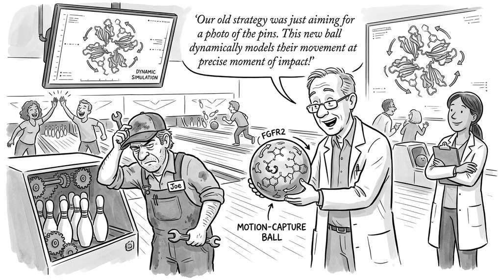
Relay Therapeutics combines molecular dynamics simulations with AI to capture protein motion, not just static structure, during drug design. Their lead program RLY-4008 (now called lirafugratinib), a selective FGFR2 inhibitor for cholangiocarcinoma, used this "dynamical pharmacology" platform to exploit a transient protein pocket invisible in static crystal structures. The compound received U.S. Food and Drug Administration (FDA) accelerated approval in 2024, demonstrating that incorporating conformational dynamics into the virtual screening pipeline can reveal binding opportunities that conventional docking on a single structure would miss entirely.
The Billion-Dollar Typo
SMILES notation is so compact that a single misplaced character can turn a life-saving drug into a completely different (and possibly toxic) molecule. The SMILES string for aspirin is CC(=O)Oc1ccccc1C(=O)O; change just the lowercase "c" atoms to uppercase "C" and you get a saturated cyclohexane derivative with none of aspirin's anti-inflammatory properties. This fragility is one reason the field is shifting from SMILES-based generative models to graph-based representations, where every generated structure is guaranteed to be a valid molecular graph by construction.
Lab: Build and Evaluate a Tanimoto Similarity Screen
Goal: Measure how well ligand-based virtual screening recovers known active compounds from a mixed library, and observe how the similarity threshold affects the precision/recall trade-off.
Tools: Python 3.9+, rdkit-pypi, matplotlib, and the TDC package (pip install PyTDC).
Setup (5 min): Load the EGFR kinase bioactivity dataset from TDC (from tdc.single_pred import HTS; data = HTS(name='sarscov2_vitro_uruber') or the EGFR set from ChEMBL). Split the known actives (half-maximal inhibitory concentration, IC50, < 1 μM) from inactives. Pick one active as your query molecule.
Experiment (15 min): Compute Morgan fingerprints (radius 2, 2048 bits) for every compound. Calculate Tanimoto similarity to the query. Sweep the threshold from 0.2 to 0.8 in steps of 0.05. At each threshold, record the number of hits, the fraction that are true actives (precision), and the fraction of all actives recovered (recall).
What to vary: (1) Fingerprint radius (1, 2, 3); (2) bit vector length (1024, 2048, 4096); (3) choice of query molecule. Observe how each parameter shifts the precision/recall curve.
What to observe: Plot precision vs. recall curves for each setting. You should find that radius 2 with 2048 bits is a robust default, that very high thresholds (> 0.7) yield high precision but miss chemically diverse actives, and that the choice of query molecule matters more than fingerprint parameters.