34.3 Equivariant Generation for 3D Structures

1. Symmetry Groups and Equivariance

Rotate a caffeine molecule 47 degrees around an arbitrary axis and slide it three angstroms to the left. Ask a standard neural network to predict its energy: you get a different answer, even though every atom is in the same relative position. The network has, in effect, confused the coordinate system with the physics. The cure starts with a precise vocabulary. A symmetry group is a set of transformations that leave some property of a system unchanged. For 3D molecular and protein structures, the relevant group is SE(3): the special Euclidean group in three dimensions, consisting of all rotations and translations. An element \(g \in \text{SE}(3)\) pairs a rotation \(R \in \text{SO}(3)\) (a \(3 \times 3\) matrix with \(R^T R = I\), \(\det R = 1\)) with a translation vector \(t \in \mathbb{R}^3\). The group acts on a point \(x \in \mathbb{R}^3\) as \(g \cdot x = Rx + t\).

SE(3) is the precise mathematical name for every rigid body motion in three dimensions. It covers rotating an object around any axis by any angle and sliding it in any direction by any distance, without stretching, squeezing, or reflecting it. SE(3) symmetry matters because the laws of physics do not depend on where you place your coordinate axes or how you orient them. A neural network that bakes in this symmetry satisfies the law automatically, rather than learning it from data. The mechanism is compositional: SE(3) transformations form a group. Any two successive rotate-and-translate operations compose into a single rotate-and-translate operation. A network layer equivariant to each individual transformation is therefore equivariant to all possible chains. Use SE(3) equivariance whenever your inputs are 3D point clouds or atomic coordinates whose physical meaning does not depend on the coordinate frame. For problems on regular grids (images, voxels) or for 2D data, simpler symmetry groups such as the Euclidean group E(2) or discrete rotations are more appropriate.

A function \(f\) is invariant under a group \(G\) if its output does not change when the input is transformed: \(f(g \cdot x) = f(x)\) for all \(g \in G\). Energy, binding affinity, and solubility are SE(3)-invariant properties: they depend on the relative positions of atoms, not their absolute coordinates.

A function \(f\) is equivariant under \(G\) if its output transforms in the same way as its input: \(f(g \cdot x) = g \cdot f(x)\) for all \(g \in G\). Forces are SE(3)-equivariant: rotating a molecule rotates the force vectors by the same rotation. For generative models, equivariance means that generating a structure and then rotating it gives the same result as rotating the noise and then generating: the generation process respects the symmetry. In short: build the symmetry in, and the network is free to learn the physics instead of the coordinate system.

Mental Model

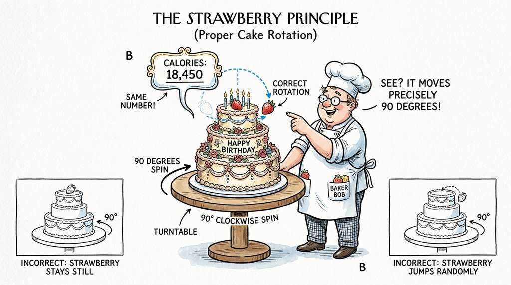
Think of a recipe for a layered cake. An invariant property is the total calorie count: no matter how you rotate the cake on the turntable, the calories stay the same. An equivariant property is the position of the strawberry on top: when you spin the turntable 90 degrees clockwise, the strawberry moves 90 degrees clockwise too. The strawberry does not stay put (that would be invariance), and it does not jump to a random new spot (that would be no symmetry at all). It tracks the rotation faithfully. An equivariant neural network is like a recipe that guarantees, by the way its steps are written, that every decoration on the cake will track the turntable spin exactly, without the baker needing to check each decoration by hand after every rotation.

2. Equivariant Graph Neural Networks

Encoding symmetry constraints into a neural network requires an architecture that operates directly on 3D atomic coordinates.

A molecular system is naturally represented as a graph: atoms are nodes with features (element type, charge) and 3D positions \(x_i \in \mathbb{R}^3\); bonds or spatial proximity define edges. An equivariant graph neural network (GNN) must update both the scalar node features \(h_i\) (invariant under SE(3)) and the coordinate positions \(x_i\) (equivariant under SE(3)) simultaneously.

The E(n) Equivariant Graph Neural Network (EGNN; Satorras et al., 2021) achieves this with a remarkably simple message passing scheme. At each layer \(\ell\), messages depend on pairwise distances (invariant) and relative positions (equivariant). Figure 34.3.1 illustrates the data flow through a single EGNN layer, showing how invariant scalar quantities and equivariant vector quantities are kept on separate tracks:

The critical design: position updates use only relative position vectors \((x_i - x_j)\) weighted by scalar functions of messages. Since relative positions are equivariant (they rotate with the system) and the weights are invariant (they depend only on distances and scalar features), the position update is equivariant by construction. No rotation matrices appear anywhere in the computation.

import torch
import torch.nn as nn
from torch_geometric.nn import MessagePassing
from torch_geometric.data import Data


class EGNNLayer(MessagePassing):
    """E(n) Equivariant Graph Neural Network layer.

    Updates both scalar features (invariant) and positions
    (equivariant) using distance-based message passing.
    """
    def __init__(self, hidden_dim: int, edge_dim: int = 0):
        super().__init__(aggr='mean')
        self.hidden_dim = hidden_dim

        # Edge message network: takes node pairs + distance + edge attrs
        self.edge_mlp = nn.Sequential(
            nn.Linear(2 * hidden_dim + 1 + edge_dim, hidden_dim),
            nn.SiLU(),
            nn.Linear(hidden_dim, hidden_dim),
            nn.SiLU()
        )
        # Position update: scalar weight from message
        self.coord_mlp = nn.Sequential(
            nn.Linear(hidden_dim, hidden_dim),
            nn.SiLU(),
            nn.Linear(hidden_dim, 1, bias=False)
        )
        # Node update network
        self.node_mlp = nn.Sequential(
            nn.Linear(2 * hidden_dim, hidden_dim),
            nn.SiLU(),
            nn.Linear(hidden_dim, hidden_dim)
        )

    def forward(self, h: torch.Tensor, pos: torch.Tensor,
                edge_index: torch.Tensor,
                edge_attr: torch.Tensor = None):
        """Update node features and positions equivariantly."""
        # Compute pairwise distances (invariant under SE(3))
        row, col = edge_index
        rel_pos = pos[row] - pos[col]              # equivariant vectors
        dist_sq = (rel_pos ** 2).sum(dim=-1, keepdim=True)  # invariant scalar

        # Build edge features
        edge_feat = torch.cat([h[row], h[col], dist_sq], dim=-1)
        if edge_attr is not None:
            edge_feat = torch.cat([edge_feat, edge_attr], dim=-1)

        # Compute messages (invariant scalars)
        msg = self.edge_mlp(edge_feat)

        # Update positions: weight relative vectors by scalar function
        coord_weight = self.coord_mlp(msg)   # scalar per edge
        pos_update = self.propagate(edge_index, x=rel_pos * coord_weight,
                                     size=None)
        pos_new = pos + pos_update

        # Update node features via aggregated messages
        msg_agg = self.propagate(edge_index, x=msg, size=None)
        h_new = self.node_mlp(torch.cat([h, msg_agg], dim=-1))
        h_new = h + h_new  # residual connection

        return h_new, pos_new

    def message(self, x_j: torch.Tensor) -> torch.Tensor:
        return x_j


class EGNN(nn.Module):
    """Multi-layer EGNN for molecular property prediction or generation."""
    def __init__(self, in_dim: int, hidden_dim: int, num_layers: int = 4,
                 edge_dim: int = 0):
        super().__init__()
        self.embedding = nn.Linear(in_dim, hidden_dim)
        self.layers = nn.ModuleList([
            EGNNLayer(hidden_dim, edge_dim) for _ in range(num_layers)
        ])
        self.output = nn.Linear(hidden_dim, hidden_dim)

    def forward(self, data: Data):
        h = self.embedding(data.x)
        pos = data.pos

        for layer in self.layers:
            h, pos = layer(h, pos, data.edge_index,
                          getattr(data, 'edge_attr', None))

        return self.output(h), pos

Beyond EGNN, more expressive equivariant architectures use higher-order representations. PaiNN (Schutt et al., 2021) maintains both scalar and vector features per node, with vector features that transform as proper 3D vectors under rotation. MACE (Batatia et al., 2022) uses equivariant message passing with body-ordered interactions and spherical harmonics (functions defined on the surface of a sphere that form a natural basis for representing directional information at each angular momentum order), achieving state-of-the-art accuracy for molecular dynamics. These architectures are the building blocks of equivariant diffusion models. EGNN's reliance on scalar messages limits its ability to distinguish molecular environments that differ only in angular arrangement; higher-order representations (vectors, tensors via spherical harmonics) capture directional information that scalars alone cannot encode, which is why production-grade force fields and generators typically use PaiNN, MACE, or NequIP rather than plain EGNN.

3. Equivariant Diffusion for Molecules

A molecular generator that ignores rotational symmetry quietly embeds coordinate-frame bias into every structure it produces, and those biases compound into unphysical strain energies when the output enters a downstream dynamics simulation. Combining equivariant GNNs with the diffusion framework from Section 34.2 yields equivariant diffusion models (EDMs; Hoogeboom et al., 2022) for 3D molecular generation. The key requirement: both the forward noising process and the learned reverse process must be SE(3) equivariant.

The forward process adds isotropic Gaussian noise to atom positions: \(x_t = \sqrt{\bar{\alpha}_t} \, x_0 + \sqrt{1 - \bar{\alpha}_t} \, \epsilon\), where \(\epsilon \sim \mathcal{N}(0, I)\). This is automatically SE(3) equivariant because Gaussian noise is rotationally symmetric (rotating the noisy molecule is the same as rotating the clean molecule and then adding noise).

The reverse process uses an equivariant GNN to predict the noise \(\epsilon_\theta(x_t, h, t)\) given noisy positions \(x_t\), atom types \(h\), and timestep \(t\). Because the EGNN's position outputs are equivariant, the predicted noise vectors transform correctly under rotation, ensuring that the denoised positions are equivariant.

One subtlety: the forward process must be translation-invariant as well. Since adding a constant translation \(t\) to all positions does not change the molecule, we work in a center-of-mass-free subspace (the subspace of \(\mathbb{R}^{3N}\) where the mean of all \(N\) atom positions is zero, effectively removing the three translational degrees of freedom from the representation) by subtracting the mean position at each step.

import torch
import torch.nn as nn
import torch.nn.functional as F


class EquivariantDiffusion(nn.Module):
    """Equivariant diffusion model for 3D molecular generation.

    Combines an EGNN denoiser with a DDPM-style diffusion process
    that respects SE(3) symmetry. Generates both atom positions
    (continuous, equivariant) and atom types (discrete, invariant).
    """
    def __init__(self, egnn: nn.Module, num_atom_types: int,
                 T: int = 1000, beta_start: float = 1e-4,
                 beta_end: float = 0.02):
        super().__init__()
        self.egnn = egnn
        self.T = T
        self.num_atom_types = num_atom_types

        betas = torch.linspace(beta_start, beta_end, T)
        alphas = 1.0 - betas
        alpha_bars = torch.cumprod(alphas, dim=0)
        self.register_buffer('alpha_bars', alpha_bars)
        self.register_buffer('betas', betas)
        self.register_buffer('alphas', alphas)

    def center_positions(self, pos: torch.Tensor,
                         batch: torch.Tensor) -> torch.Tensor:
        """Remove center of mass (translation invariance)."""
        # Compute per-graph mean and subtract
        from torch_geometric.utils import scatter
        mean = scatter(pos, batch, dim=0, reduce='mean')
        return pos - mean[batch]

    def forward_diffusion(self, pos: torch.Tensor, t: torch.Tensor,
                          batch: torch.Tensor):
        """Add noise to positions, maintaining center-of-mass zero."""
        alpha_bar = self.alpha_bars[t]

        # Per-node alpha_bar based on which graph each node belongs to
        alpha_bar_node = alpha_bar[batch].unsqueeze(-1)

        noise = torch.randn_like(pos)
        noise = self.center_positions(noise, batch)  # center noise too

        pos_noisy = torch.sqrt(alpha_bar_node) * pos + \
                    torch.sqrt(1 - alpha_bar_node) * noise
        return pos_noisy, noise

    def training_loss(self, data):
        """Compute equivariant denoising loss."""
        pos = self.center_positions(data.pos, data.batch)
        batch_size = data.batch.max().item() + 1

        # Sample random timesteps (one per graph)
        t = torch.randint(0, self.T, (batch_size,), device=pos.device)

        # Add noise to positions
        pos_noisy, noise_target = self.forward_diffusion(pos, t, data.batch)

        # Create noisy data object
        data_noisy = data.clone()
        data_noisy.pos = pos_noisy

        # Predict noise using equivariant network
        h_pred, pos_pred = self.egnn(data_noisy)

        # The position output predicts the noise direction (equivariant)
        noise_pred = pos_pred - pos_noisy  # predicted noise = output - input
        noise_pred = self.center_positions(noise_pred, data.batch)

        # MSE loss on noise prediction
        pos_loss = F.mse_loss(noise_pred, noise_target)

        return pos_loss

    @torch.no_grad()
    def sample(self, num_atoms_per_mol: list, atom_types: torch.Tensor,
               edge_index: torch.Tensor, batch: torch.Tensor,
               device: torch.device):
        """Generate 3D molecular structures via reverse diffusion."""
        total_atoms = sum(num_atoms_per_mol)

        # Start from centered Gaussian noise
        pos = torch.randn(total_atoms, 3, device=device)
        pos = self.center_positions(pos, batch)

        for t_val in reversed(range(self.T)):
            t = torch.full((len(num_atoms_per_mol),), t_val,
                          device=device, dtype=torch.long)

            # Build data object with current noisy positions
            from torch_geometric.data import Data
            data_t = Data(x=atom_types, pos=pos,
                         edge_index=edge_index, batch=batch)

            # Predict noise
            h_out, pos_out = self.egnn(data_t)
            noise_pred = pos_out - pos
            noise_pred = self.center_positions(noise_pred, batch)

            # Reverse step
            alpha_t = self.alphas[t_val]
            alpha_bar_t = self.alpha_bars[t_val]
            beta_t = self.betas[t_val]

            pos = (1 / torch.sqrt(alpha_t)) * (
                pos - (beta_t / torch.sqrt(1 - alpha_bar_t)) * noise_pred
            )

            if t_val > 0:
                noise = torch.randn_like(pos)
                noise = self.center_positions(noise, batch)
                pos = pos + torch.sqrt(beta_t) * noise

            pos = self.center_positions(pos, batch)  # maintain COM = 0

        return pos

4. Protein Backbone Generation

Protein backbone generation is perhaps the most impactful application of equivariant generative models. A protein backbone is defined by the 3D coordinates of four atoms per residue (N, C\(_\alpha\), C, O), or equivalently by a rigid body frame (rotation + translation) at each residue. The design task: generate a backbone structure that, when the side chains are added and the sequence is designed, will fold into the intended 3D structure and perform a desired function. Because each residue's orientation is a rotation (an element of SO(3), a curved manifold rather than a flat Euclidean space), the simple Gaussian noising from Section 3 no longer applies directly; the protein backbone generators below each develop a manifold-aware noise process tailored to SE(3).

Three landmark systems have tackled this problem with different generative frameworks, each choosing a distinct strategy for handling the SE(3) manifold. Figure 34.3.2 summarizes the three approaches side by side:

RFDiffusion (Watson et al., 2023) fine-tunes the RoseTTAFold structure prediction network as a denoiser. The key insight: a structure prediction network already knows what valid protein structures look like, so it can serve as a powerful prior for denoising. (This is why RFDiffusion succeeded where earlier protein generators struggled: it starts from a network that already encodes the grammar of protein folds, turning a generation problem into a much simpler denoising problem.) RFDiffusion operates on residue frames (rotation matrices + translation vectors), running diffusion on both the rotational (SO(3)) and translational (\(\mathbb{R}^3\)) components. It supports conditioning on functional motifs (specific geometric arrangements of a few key residues, such as a catalytic triad or a binding pocket, that define the protein's biological function): given a binding site geometry, RFDiffusion generates a complete protein backbone that scaffolds (builds a full supporting structure around) that motif. Experimentally validated designs include novel protein binders for influenza hemagglutinin and SARS-CoV-2 receptor binding domain.

Diffusion and Flow Matching on the SE(3) Manifold

FrameDiff (Yim et al., 2023) runs diffusion directly on the SE(3) manifold, representing each residue as a frame \(T_i = (R_i, t_i) \in \text{SE}(3)\). The forward process adds rotational noise via the IGSO3 distribution (the isotropic Gaussian distribution on the SO(3) rotation group, which generalizes the familiar Gaussian to the curved manifold of 3D rotations) and translational noise via standard Gaussian. An Invariant Point Attention (IPA) network, where IPA is a transformer attention mechanism that computes attention scores using both sequence features and 3D point coordinates in a way that is invariant to global rigid body transformations, inspired by AlphaFold2 predicts frame updates in the reverse direction, guaranteeing that every generated structure lies on the correct manifold.

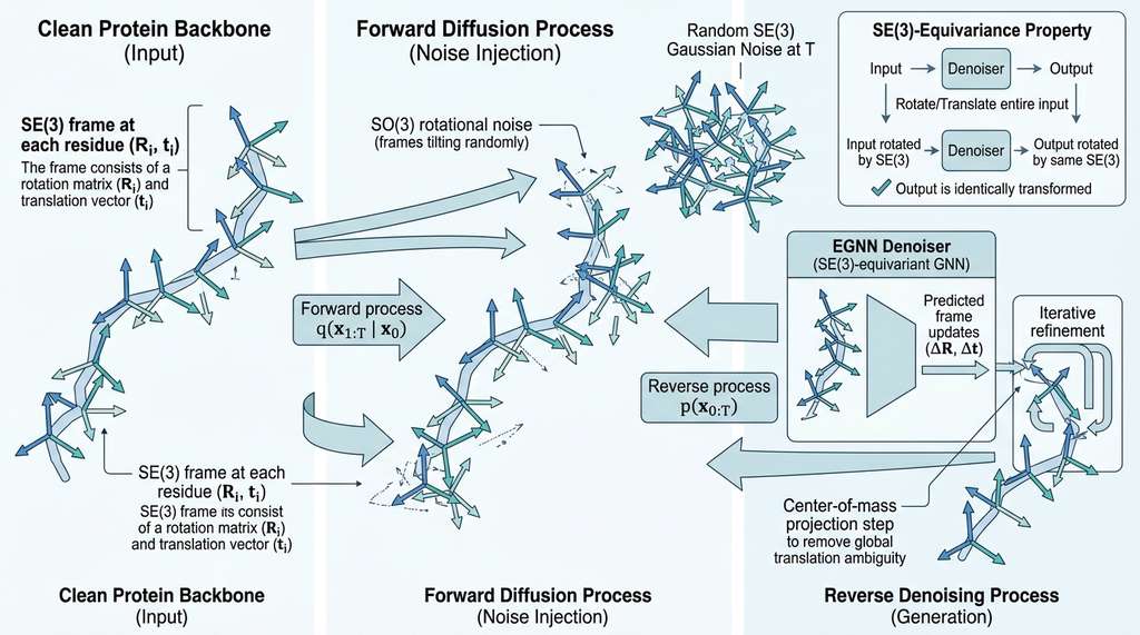
FoldFlow (Bose et al., 2024) applies flow matching on SE(3). Instead of diffusing and denoising, it learns a velocity field that transports random frames to valid protein backbone frames along geodesic paths (shortest curves connecting two points on a curved manifold, generalizing the concept of a straight line to non-Euclidean geometry) on the SE(3) manifold. The advantage: flow matching requires only defining interpolation paths, which are simpler on manifolds than defining a full noising process. FoldFlow achieves comparable designability (the fraction of generated backbones for which a sequence can be computationally designed that folds back into the intended structure, as verified by a structure predictor such as AlphaFold2) to RFDiffusion and FrameDiff with fewer sampling steps. Figure 34.3.3 illustrates SE(3)-equivariant diffusion process for protein backbone generation.

5. Structure Prediction as Generation

RFDiffusion, FrameDiff, and FoldFlow all generate novel backbones, but each relies on a network that already understands what valid protein structures look like, blurring the line between predicting a structure and generating one.

Structure prediction (given a sequence, predict the 3D structure) and structure generation (sample novel 3D structures) are two sides of the same coin. AlphaFold2 (Jumper et al., 2021) solved single-chain structure prediction with a deterministic architecture; subsequent work has reframed the problem as generative modeling to handle the inherent uncertainty in flexible regions and multi-chain complexes.

Boltz-1 (Wohlwend et al., 2024) is an open-weight biomolecular structure prediction model that uses diffusion to predict structures of protein-ligand, protein-nucleic acid, and protein-protein complexes. Unlike AlphaFold2's deterministic prediction, Boltz-1's diffusion-based approach naturally produces an ensemble of structures, capturing conformational flexibility. On standard benchmarks, it reportedly achieves accuracy competitive with AlphaFold3 while being fully open-source.

Chai-1 (Chai Discovery, 2024) similarly uses a diffusion-based architecture for multi-chain complex prediction, with additional capabilities for predicting the effects of mutations and post-translational modifications. The generative framing means that sampling multiple structures from the model approximates the Boltzmann ensemble (the probability distribution over molecular conformations weighted by \(e^{-E/k_BT}\), where lower-energy states are exponentially more probable, as described by statistical mechanics), connecting back to the statistical mechanics foundations from Chapter 43.

6. Beyond Proteins: Crystals, Conformers, and Materials

Proteins are the showcase application, but the same principle (match the network's symmetry to the physics of the domain) applies wherever 3D structure determines function.

The equivariant diffusion framework extends beyond proteins to any domain with 3D structure and physical symmetries. Crystal diffusion (CDVAE; Xie et al., 2022) generates crystal structures by diffusing atom positions within a periodic unit cell, respecting the additional periodic boundary symmetry. Conformer generation (GeoDiff; Xu et al., 2022) produces 3D molecular conformations from 2D molecular graphs, treating the problem as conditional generation. Materials design (MatterGen; Zeni et al., 2024) uses diffusion to jointly generate atom types, positions, and lattice parameters for novel inorganic materials, conditioned on target properties like formation energy or band gap.

Each domain adds its own symmetry requirements: crystals need periodic equivariance, molecular conformers need chirality preservation, and materials need space group consistency. The pattern is consistent: identify the symmetry group, build an equivariant network, and run diffusion or flow matching in the symmetry-respecting subspace.

import e3nn
from e3nn import o3
from e3nn.nn.models.gate_points_2101 import Network

# Define irreducible representations
irreps_in = "5x0e"      # 5 scalar features (even parity)
irreps_hidden = "32x0e + 16x1o + 8x2e"  # scalars + vectors + rank-2 tensors
irreps_out = "1x1o"     # output: 3D vector (force, velocity, noise)

# Build equivariant network with spherical harmonics
model = Network(
    irreps_in=irreps_in,
    irreps_hidden=irreps_hidden,
    irreps_out=irreps_out,
    irreps_node_attr="0e",
    irreps_edge_attr=o3.Irreps.spherical_harmonics(lmax=2),
    layers=4,
    max_radius=5.0,
    number_of_basis=8,
    radial_layers=2,
    radial_neurons=64,
    num_neighbors=12.0,
    num_nodes=20.0
)
# Output transforms as a proper 3D vector under rotation

Exercises

1. (Conceptual) Explain why molecular force fields must be SE(3) equivariant but molecular energies must be SE(3) invariant. If you built a generative model that predicted energies equivariantly (incorrectly), what physical artifacts would you expect in the generated structures? How would these artifacts manifest in a downstream molecular dynamics simulation?
2. (Coding) Implement the EGNN from this section and verify its equivariance empirically. Generate a random molecular graph with positions in \(\mathbb{R}^3\), process it through the network, then rotate all positions by a random rotation matrix and process again. Verify that the output positions differ by exactly the same rotation (up to floating-point precision). Measure the equivariance error as \(\|R \cdot f(x) - f(R \cdot x)\|\) for 100 random rotations. What is the typical error magnitude?
3. (Analysis) Compare the EGNN architecture with a standard GNN (no equivariance) on the QM9 molecular property prediction benchmark (a dataset of ~134,000 small organic molecules with up to 9 heavy atoms, each annotated with 13 quantum chemical properties computed via density functional theory) (available via PyTorch Geometric). Train both models to predict the highest occupied molecular orbital / lowest unoccupied molecular orbital (HOMO-LUMO) gap. Does the equivariant model achieve lower test error? Does it converge faster? How does the advantage change if you add random rotation augmentation to the standard GNN's training data?