49.3 Materials Design and Universal Force Fields

1. Crystal Structure and the Materials Design Problem

A crystal is defined by its unit cell: a parallelepiped specified by lattice vectors \(\mathbf{a}_1, \mathbf{a}_2, \mathbf{a}_3 \in \mathbb{R}^3\) and a set of atoms at fractional coordinates (each component ranges from 0 to 1, expressing position as a fraction of the corresponding lattice vector) within that cell. The lattice vectors determine the cell shape and volume; the fractional coordinates determine the atomic arrangement. Together, they define a periodic structure that tiles all of 3D space.

The materials design problem is: given a target property \(y^*\) (e.g., band gap of 1.5 eV for a solar cell absorber), find a crystal structure \((L, \mathbf{f})\) such that \(y(L, \mathbf{f}) \approx y^*\), where \(L = [\mathbf{a}_1, \mathbf{a}_2, \mathbf{a}_3]\) is the lattice matrix and \(\mathbf{f} = [\mathbf{f}_1, \ldots, \mathbf{f}_n]\) are fractional coordinates. The property function \(y(\cdot)\) is computed by DFT or measured experimentally. The search space has several features that distinguish it from molecular design:

• Periodicity: the structure repeats infinitely, so properties depend on the unit cell and its periodic images.
• Symmetry: crystals belong to one of 230 space groups (the distinct symmetry patterns, combining rotations, reflections, and translations, that a three-dimensional periodic structure can exhibit), imposing constraints on allowed atomic positions.
• Composition: unlike organic molecules (dominated by C, H, N, O, S), materials span the entire periodic table, including transition metals, rare earths, and actinides.
• Stability: a generated structure must be thermodynamically stable (or at least metastable, meaning it sits in a local energy minimum but not the global one, so it can persist indefinitely under normal conditions) to be experimentally realizable.

2. Crystal Structure Generation with MatterGen

MatterGen (Zeni et al., 2025) is a diffusion model for generating novel crystal structures. It operates on three types of variables simultaneously: atom types (categorical), atom positions (continuous, with periodic boundary conditions), and lattice parameters (continuous). The diffusion process adds noise to all three components, and the denoising network learns to recover valid crystal structures from noise.

The forward process for atomic positions must respect periodicity. MatterGen uses a wrapped Gaussian distribution on the unit torus \([0, 1)^3\) for fractional coordinates:

Mental Model

Think of the wrapped Gaussian diffusion like smearing paint on the surface of a globe. If you blur a dot of paint on a flat sheet, the color simply fades outward and eventually disappears at the edges. But on a globe, paint that drifts past one side reappears on the opposite side, because the surface wraps around. Similarly, when MatterGen adds noise to an atom sitting near the edge of the unit cell (say at fractional coordinate 0.98), that noise must wrap around so the atom can diffuse to position 0.02 on the other side, because in a crystal those two positions are physically adjacent. The "unit torus" is the mathematical equivalent of this globe-like wrapping, applied independently along each of the three crystal axes.

This wrapping ensures that positions near cell boundaries diffuse correctly across periodic boundaries. For atom types, MatterGen uses a discrete diffusion process that gradually corrupts atom labels toward a uniform distribution over element types. For lattice parameters, standard Gaussian diffusion on the 6-dimensional parameterization (three lengths and three angles) is used.

MatterGen can be conditioned on desired properties (e.g., "generate a crystal with band gap between 1.0 and 2.0 eV") by training with classifier-free guidance. The conditioning signal is dropped randomly during training, and at inference time, the model interpolates between the unconditional and conditional score:

where \(w\) is the guidance weight and \(c\) is the conditioning signal. Higher \(w\) produces structures that more closely match the condition but with reduced diversity. In short: a single diffusion model, trained to denoise atom types, positions, and lattice parameters simultaneously, turns "generate a crystal with this property" from a years-long experimental search into a minutes-long sampling loop.

from pymatgen.core import Structure, Lattice
import numpy as np


def create_crystal_structure(
    species: list[str],
    lattice_params: dict,
    frac_coords: np.ndarray,
) -> Structure:
    """Create a pymatgen Structure from generated parameters.

    This is the output format for MatterGen and similar crystal
    generators. Pymatgen handles symmetry analysis, property
    computation, and file I/O.

    Args:
        species: List of element symbols, e.g. ["Si", "O", "O"].
        lattice_params: Dict with 'a', 'b', 'c', 'alpha', 'beta', 'gamma'.
        frac_coords: (n_atoms, 3) fractional coordinates in [0, 1).

    Returns:
        pymatgen Structure object.
    """
    lattice = Lattice.from_parameters(
        a=lattice_params["a"],
        b=lattice_params["b"],
        c=lattice_params["c"],
        alpha=lattice_params["alpha"],
        beta=lattice_params["beta"],
        gamma=lattice_params["gamma"],
    )
    structure = Structure(lattice, species, frac_coords)
    return structure


def validate_crystal(structure: Structure,
                     min_distance: float = 0.5) -> dict:
    """Validate a generated crystal structure.

    Checks for physically reasonable interatomic distances,
    valid composition, and structural sanity.

    Args:
        structure: pymatgen Structure to validate.
        min_distance: Minimum allowed interatomic distance (Angstroms).

    Returns:
        Dict with validation results.
    """
    # Check minimum interatomic distance
    dist_matrix = structure.distance_matrix
    np.fill_diagonal(dist_matrix, np.inf)
    min_dist = dist_matrix.min()

    # Check composition validity
    comp = structure.composition
    is_charge_balanced = abs(comp.oxi_state_guesses()[0].total_charge
                            if comp.oxi_state_guesses() else 1.0) < 0.1

    # Check density (typical solids: 1-25 g/cm^3)
    density = structure.density

    return {
        "valid_distances": min_dist > min_distance,
        "min_distance_angstrom": round(min_dist, 3),
        "charge_balanced": is_charge_balanced,
        "density_g_cm3": round(density, 3),
        "reasonable_density": 0.5 < density < 30.0,
        "n_atoms": len(structure),
        "formula": str(comp.reduced_formula),
        "space_group": structure.get_space_group_info()[0],
    }


# Example: create and validate a generated perovskite structure
perovskite = create_crystal_structure(
    species=["Ba", "Ti", "O", "O", "O"],
    lattice_params={
        "a": 4.01, "b": 4.01, "c": 4.01,
        "alpha": 90, "beta": 90, "gamma": 90,
    },
    frac_coords=np.array([
        [0.0, 0.0, 0.0],   # Ba
        [0.5, 0.5, 0.5],   # Ti
        [0.5, 0.5, 0.0],   # O
        [0.5, 0.0, 0.5],   # O
        [0.0, 0.5, 0.5],   # O
    ]),
)
print(validate_crystal(perovskite))

3. Universal Machine-Learned Force Fields

Generating candidate crystals, as MatterGen does, is only half the problem; every candidate must be evaluated for thermodynamic stability, and that evaluation is dominated by the cost of computing energies and forces.

Without a fast substitute for quantum-mechanical calculation, most computationally generated crystals are never evaluated: they accumulate in databases as unscored proposals, and the best material in a batch of 10,000 candidates can remain buried simply because no one could afford the CPU time to check its stability.

The bottleneck in computational materials science is the energy calculation. DFT computes the total energy \(E(\{\mathbf{r}_i, Z_i\})\) of a collection of atoms from quantum mechanics, but it scales as \(O(N^3)\) with the number of electrons \(N\), making simulations of more than a few hundred atoms prohibitively expensive. Classical force fields are fast (\(O(N)\)) but require hand-tuned parameters for each new chemical system.

From Classical to Learned Potentials

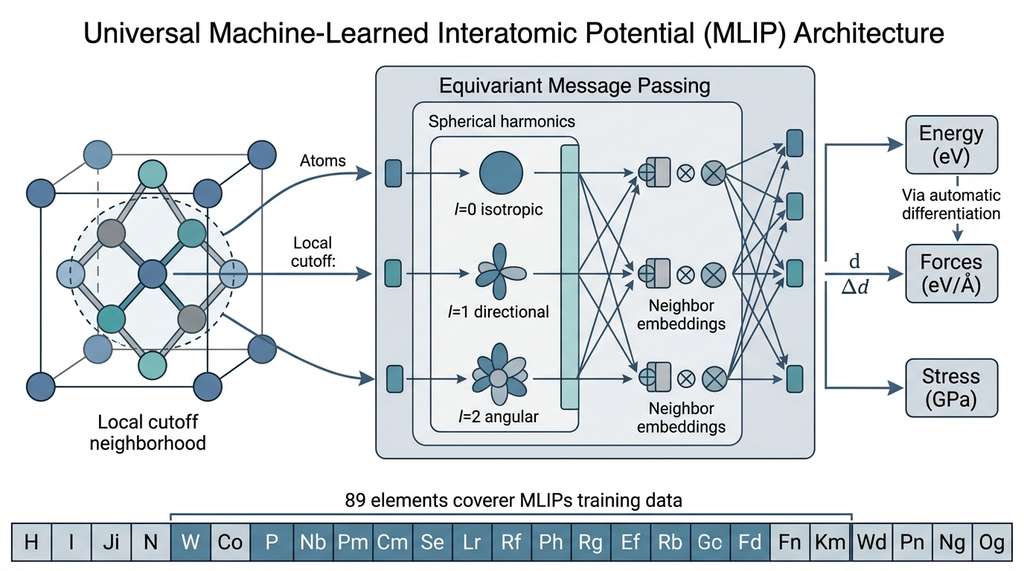
Machine-learned interatomic potentials (MLIPs) bridge this gap. They learn the mapping from atomic positions to energies and forces from DFT training data, achieving near-DFT accuracy at a fraction of the cost. The key insight is that the total energy decomposes into local atomic contributions:

A universal MLIP is a single neural network trained on DFT calculations spanning most of the periodic table. It predicts energies and forces for any combination of elements without retraining. Traditional force fields require laboriously reparameterizing every new chemical system (a new alloy, a new oxide), blocking rapid exploration; a universal MLIP removes that bottleneck. The network learns element-specific embeddings and interaction rules from a massive, chemically diverse training set (such as the 150,000+ structures in the Materials Project). It generalizes to unseen compositions the same way a language model generalizes to unseen sentences. Use a universal MLIP when you need approximate DFT-quality energies and forces across many chemistries at screening speed; fall back to system-specific MLIPs or full DFT when you need sub-meV accuracy on a single well-defined system.

where \(\varepsilon_i\) is the energy contribution of atom \(i\), which depends only on atoms within a local cutoff neighborhood \(\mathcal{N}(i)\). Forces are obtained as the negative gradient: \(\mathbf{F}_i = -\nabla_{\mathbf{r}_i} E\). The neural network parameterizes \(\varepsilon_i\); the force prediction comes for free through automatic differentiation. Figure 49.3.1 illustrates Universal machine-learned interatomic potential (MLIP) architecture.

3.1 MACE-MP-0: A Foundation Model for Atomistic Simulation

MACE-MP-0 (Batatia et al., 2024) is a universal MLIP trained on the Materials Project database. It covers 89 elements across 150,000+ structures (circa 2024). The MACE (Multi-ACE) architecture represents atomic environments through equivariant message passing with higher-order tensor products. MACE's principal design difference from earlier MLIPs (SchNet, DimeNet, NequIP) is its explicit encoding of many-body interactions through higher-order tensor products (as of 2025, successors such as MACE-MP-0b and MACE-MPA-0 further improve accuracy and coverage): while pairwise models capture bond stretching, MACE captures the angular and dihedral correlations that determine crystal stability.

The MACE energy model computes atomic energies through \(L\) layers of equivariant message passing. Each layer constructs messages using tensor products of spherical harmonics (a family of basis functions defined on the surface of a sphere that decompose angular information into components of increasing directional complexity), which encode the angular distribution of neighbors:

where \(Y_l^m\) are spherical harmonics evaluated on the unit direction vector \(\hat{\mathbf{r}}_{ij}\), and \(\phi^{(l)}\) is a learnable function involving equivariant tensor products. The spherical harmonics basis naturally captures angular information: \(l=0\) gives isotropic (distance-only) information, \(l=1\) gives directional information, and \(l \geq 2\) captures higher-order angular correlations.

from mace.calculators import mace_mp
from ase import Atoms
from ase.optimize import BFGS
from ase.constraints import UnitCellFilter
import numpy as np


def relax_structure_mace(
    atoms: Atoms,
    fmax: float = 0.01,
    max_steps: int = 500,
    relax_cell: bool = True,
    model: str = "medium",
) -> dict:
    """Relax an atomic structure using MACE-MP-0.

    Optimizes atomic positions (and optionally cell shape)
    to minimize the total energy predicted by the universal
    MACE potential.

    Args:
        atoms: ASE Atoms object to relax.
        fmax: Force convergence criterion (eV/Angstrom).
        max_steps: Maximum optimization steps.
        relax_cell: Whether to also relax the unit cell.
        model: MACE model size ("small", "medium", "large").

    Returns:
        Dict with relaxed structure, energy, forces, and stress.
    """
    # Load the pre-trained universal MACE potential
    calc = mace_mp(model=model, default_dtype="float64")
    atoms.calc = calc

    # Initial energy and forces
    e_initial = atoms.get_potential_energy()
    f_max_initial = np.max(np.abs(atoms.get_forces()))

    # Set up optimizer
    if relax_cell:
        # UnitCellFilter allows simultaneous cell + position relaxation
        filtered = UnitCellFilter(atoms)
        optimizer = BFGS(filtered, logfile="relax.log")
    else:
        optimizer = BFGS(atoms, logfile="relax.log")

    # Run relaxation
    optimizer.run(fmax=fmax, steps=max_steps)
    converged = optimizer.converged()

    # Final properties
    energy = atoms.get_potential_energy()
    forces = atoms.get_forces()
    stress = atoms.get_stress() if relax_cell else None

    return {
        "converged": converged,
        "n_steps": optimizer.nsteps,
        "energy_eV": round(energy, 6),
        "energy_per_atom_eV": round(energy / len(atoms), 6),
        "energy_change_eV": round(energy - e_initial, 6),
        "max_force_eV_A": round(np.max(np.linalg.norm(forces, axis=1)), 6),
        "stress_GPa": np.round(stress * 160.2, 3).tolist() if stress is not None else None,
        "volume_A3": round(atoms.get_volume(), 3),
        "atoms": atoms,
    }


# Example: relax a perovskite structure
from ase.build import bulk

# Create BaTiO3 perovskite
atoms = bulk("BaTiO3", crystalstructure="perovskite", a=4.01)
result = relax_structure_mace(atoms, relax_cell=True)
print(f"Energy: {result['energy_per_atom_eV']:.4f} eV/atom, "
      f"converged in {result['n_steps']} steps")

3.2 CHGNet: Charge-Informed Neural Network Potential

MACE-MP-0 captures geometry and angular correlations, but it treats all oxidation states of an element identically; for materials whose properties hinge on charge state, a potential that explicitly models oxidation is essential.

CHGNet (Deng et al., 2023) incorporates atomic charge information directly into the potential. Oxidation states govern the behavior of transition metal oxides, battery materials, and catalysts: iron oxide alone spans FeO (Fe\(^{2+}\)), Fe\(_2\)O\(_3\) (Fe\(^{3+}\)), and Fe\(_3\)O\(_4\) (mixed valence), each with distinct properties. By predicting both energies and magnetic moments, CHGNet distinguishes oxidation states that geometry-only potentials conflate.

from chgnet.model import CHGNet
from chgnet.model.dynamics import MolecularDynamics
from pymatgen.core import Structure
import numpy as np


def predict_properties_chgnet(
    structure: Structure,
) -> dict:
    """Predict material properties using CHGNet.

    CHGNet predicts energies, forces, stresses, and magnetic
    moments (proxy for oxidation states) in a single forward pass.

    Args:
        structure: pymatgen Structure object.

    Returns:
        Dict with predicted properties.
    """
    model = CHGNet.load()
    prediction = model.predict_structure(structure)

    return {
        "energy_per_atom_eV": round(prediction["e"], 4),
        "forces_eV_A": prediction["f"].tolist(),
        "stress_GPa": prediction["s"].tolist(),
        "magmoms": prediction["m"].tolist(),
        "max_force": round(np.max(np.abs(prediction["f"])), 4),
    }


def run_md_chgnet(
    structure: Structure,
    temperature: float = 300.0,
    timestep: float = 2.0,
    n_steps: int = 1000,
    ensemble: str = "nvt_nose_hoover",
) -> dict:
    """Run molecular dynamics with CHGNet.

    Simulates atomic motion at finite temperature to assess
    thermal stability and phase transitions.

    Args:
        structure: Initial pymatgen Structure.
        temperature: Temperature in Kelvin.
        timestep: MD timestep in femtoseconds.
        n_steps: Number of MD steps.
        ensemble: Thermodynamic ensemble.

    Returns:
        Dict with trajectory summary and stability assessment.
    """
    model = CHGNet.load()

    md = MolecularDynamics(
        atoms=structure,
        model=model,
        ensemble=ensemble,
        temperature=temperature,
        timestep=timestep,
        logfile="md.log",
        trajectory="md_trajectory.traj",
    )

    md.run(n_steps)

    # Analyze trajectory for stability
    energies = md.get_energies()
    temperatures = md.get_temperatures()

    # Check if structure remained intact
    final_structure = md.atoms.get_structure()
    initial_volume = structure.volume
    final_volume = final_structure.volume
    volume_change = abs(final_volume - initial_volume) / initial_volume

    return {
        "mean_energy_eV": round(np.mean(energies), 4),
        "energy_std_eV": round(np.std(energies), 4),
        "mean_temperature_K": round(np.mean(temperatures), 1),
        "volume_change_fraction": round(volume_change, 4),
        "thermally_stable": volume_change < 0.1,  # <10% volume change
        "n_steps_completed": n_steps,
    }

4. Property Prediction Across the Periodic Table

With universal potentials that can score any crystal in milliseconds, the remaining challenge is assembling generation, relaxation, and stability analysis into a single automated pipeline that ranks thousands of candidates without manual intervention.

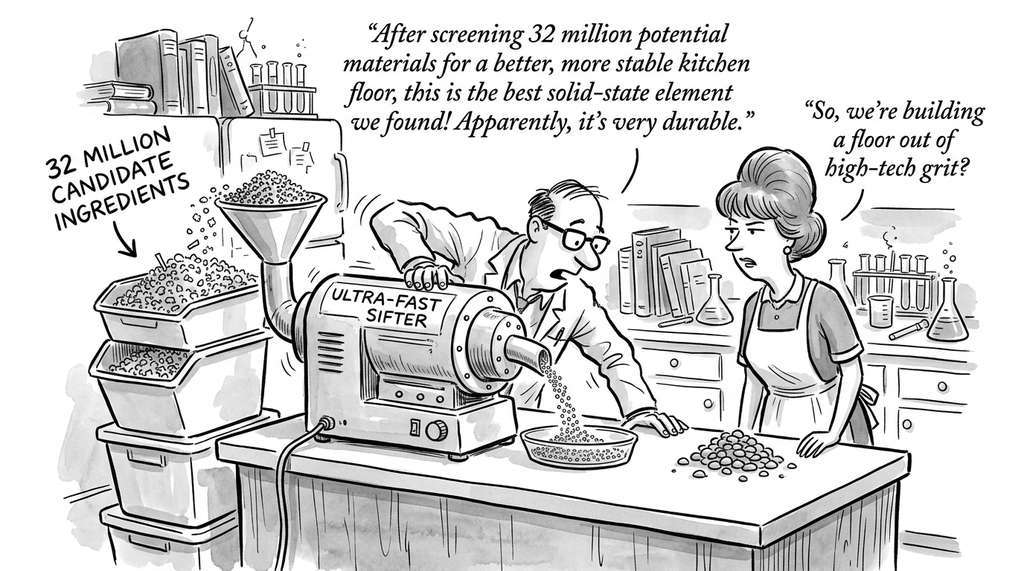
Universal force fields enable a new mode of materials discovery: instead of computing properties one material at a time, we can screen thousands of candidates in hours. As illustrated in the materials screening pipeline diagram (Figure 49.3.2), the workflow combines generation, relaxation, and property prediction in a sequence of progressively narrower filters:

from dataclasses import dataclass
from pymatgen.core import Structure
from pymatgen.analysis.phase_diagram import PhaseDiagram
from pymatgen.entries.computed_entries import ComputedStructureEntry
import numpy as np
import json
from pathlib import Path


@dataclass
class MaterialCandidate:
    """A candidate material with predicted properties."""
    formula: str
    structure: Structure
    energy_per_atom: float
    energy_above_hull: float   # Thermodynamic stability metric
    band_gap: float            # Predicted electronic band gap
    bulk_modulus: float        # Mechanical stiffness
    is_stable: bool


def screen_materials(
    candidates: list[Structure],
    competing_entries: list,  # Known phases for hull calculation
    property_model,           # ML model for band gap, modulus
    e_above_hull_cutoff: float = 0.1,  # eV/atom
) -> list[MaterialCandidate]:
    """Screen a batch of candidate materials for stability and properties.

    Args:
        candidates: List of pymatgen Structures to evaluate.
        competing_entries: Known ComputedEntries for phase diagram.
        property_model: Model predicting band gap and bulk modulus.
        e_above_hull_cutoff: Maximum energy above hull (eV/atom).

    Returns:
        Sorted list of MaterialCandidate (most stable first).
    """
    results = []

    for struct in candidates:
        # 1. Predict energy with MACE
        energy = predict_energy_mace(struct)
        energy_per_atom = energy / len(struct)

        # 2. Compute energy above convex hull
        entry = ComputedStructureEntry(
            struct, energy,
            parameters={"potcar_symbols": ["PBE"] * len(struct.species)},
        )
        all_entries = competing_entries + [entry]
        try:
            pd = PhaseDiagram(all_entries)
            e_above_hull = pd.get_e_above_hull(entry)
        except Exception:
            e_above_hull = float("inf")

        # 3. Predict properties (band gap, bulk modulus)
        props = property_model.predict(struct)

        is_stable = e_above_hull < e_above_hull_cutoff

        results.append(MaterialCandidate(
            formula=struct.composition.reduced_formula,
            structure=struct,
            energy_per_atom=round(energy_per_atom, 4),
            energy_above_hull=round(e_above_hull, 4),
            band_gap=round(props.get("band_gap", 0.0), 3),
            bulk_modulus=round(props.get("bulk_modulus", 0.0), 1),
            is_stable=is_stable,
        ))

    # Sort by energy above hull (most stable first)
    results.sort(key=lambda r: r.energy_above_hull)

    n_stable = sum(1 for r in results if r.is_stable)
    print(f"Screened {len(results)} candidates: "
          f"{n_stable} within {e_above_hull_cutoff} eV/atom of hull")

    return results


def predict_energy_mace(structure: Structure) -> float:
    """Predict total energy using MACE-MP-0 (wrapper)."""
    from mace.calculators import mace_mp
    from ase.io import read as ase_read
    from pymatgen.io.ase import AseAtomsAdaptor

    atoms = AseAtomsAdaptor.get_atoms(structure)
    calc = mace_mp(model="medium", default_dtype="float64")
    atoms.calc = calc
    return atoms.get_potential_energy()

# As of 2024, the mp-api package replaces the legacy pymatgen.ext.matproj
# interface. Install via: pip install mp-api
from mp_api.client import MPRester
from pymatgen.analysis.phase_diagram import PhaseDiagram, PDPlotter

with MPRester("YOUR_API_KEY") as mpr:
    entries = mpr.get_entries_in_chemsys(["Li", "Fe", "O"])

pd = PhaseDiagram(entries)
plotter = PDPlotter(pd)
plotter.get_plot()  # Ternary phase diagram in one line

5. Autonomous Chemistry Laboratories

The ultimate expression of AI-driven materials discovery is the autonomous laboratory: a system that designs experiments, executes them on robotic platforms, analyzes results, and plans the next round without human intervention. This connects directly to the self-driving lab paradigm covered in Chapter 55, with chemistry-specific instrumentation and constraints.

An autonomous chemistry lab integrates four components. The brain is a Bayesian optimization (BO) loop (from Chapter 45) that selects which experiments to run, balancing exploration of unknown regions with exploitation of promising leads. The hands are robotic platforms (liquid handlers, automated reactors, plate readers) that execute experiments. The eyes are analytical instruments (mass spectrometry, nuclear magnetic resonance (NMR), X-ray diffraction) that characterize products. The memory is a structured database (the experiment registry from Chapter 47) that records every decision, observation, and result for reproducibility.

from dataclasses import dataclass, field
from datetime import datetime
import json
from pathlib import Path
import numpy as np


@dataclass
class LabExperiment:
    """A single experiment in an autonomous chemistry campaign."""
    experiment_id: str
    parameters: dict          # Reagent amounts, temperature, time, etc.
    predicted_outcome: float  # Surrogate prediction
    acquisition_value: float  # Acquisition function value
    measured_outcome: float | None = None
    status: str = "planned"   # planned -> running -> completed -> failed
    timestamp: str = field(
        default_factory=lambda: datetime.now().isoformat()
    )


class AutonomousChemistryLoop:
    """Closed-loop autonomous chemistry optimization.

    Integrates Bayesian optimization with robotic execution
    and analytical measurement in a self-driving loop.
    """

    def __init__(
        self,
        parameter_space: dict,   # {name: (low, high)} for each parameter
        objective_name: str,     # What we are optimizing
        output_dir: str,
        batch_size: int = 4,     # Experiments per round (parallel)
    ):
        self.param_space = parameter_space
        self.objective = objective_name
        self.output_dir = Path(output_dir)
        self.output_dir.mkdir(parents=True, exist_ok=True)
        self.batch_size = batch_size
        self.experiments: list[LabExperiment] = []
        self.round_num = 0

    def suggest_next_batch(self) -> list[dict]:
        """Use Bayesian optimization to suggest the next experiments.

        Returns list of parameter dicts for the next batch.
        """
        from botorch.models import SingleTaskGP
        from botorch.acquisition import ExpectedImprovement
        from botorch.optim import optimize_acqf
        from gpytorch.mlls import ExactMarginalLogLikelihood
        import torch

        completed = [e for e in self.experiments
                     if e.status == "completed"]

        if len(completed) < 3:
            # Not enough data for Gaussian process (GP): use random sampling
            return self._random_batch()

        # Prepare training data
        param_names = sorted(self.param_space.keys())
        bounds = torch.tensor([
            [self.param_space[p][0] for p in param_names],
            [self.param_space[p][1] for p in param_names],
        ], dtype=torch.float64)

        X = torch.tensor([
            [e.parameters[p] for p in param_names]
            for e in completed
        ], dtype=torch.float64)
        Y = torch.tensor([
            [e.measured_outcome] for e in completed
        ], dtype=torch.float64)

        # Normalize
        X_norm = (X - bounds[0]) / (bounds[1] - bounds[0])

        # Fit GP surrogate
        gp = SingleTaskGP(X_norm, Y)
        mll = ExactMarginalLogLikelihood(gp.likelihood, gp)
        from botorch.fit import fit_gpytorch_mll
        fit_gpytorch_mll(mll)

        # Optimize acquisition function
        ei = ExpectedImprovement(gp, best_f=Y.max())
        candidates, acq_values = optimize_acqf(
            ei, bounds=torch.stack([
                torch.zeros(len(param_names)),
                torch.ones(len(param_names)),
            ]),
            q=self.batch_size,
            num_restarts=10,
            raw_samples=256,
        )

        # Denormalize
        candidates_real = candidates * (bounds[1] - bounds[0]) + bounds[0]

        batch = []
        for i in range(self.batch_size):
            params = {
                p: round(float(candidates_real[i, j]), 4)
                for j, p in enumerate(param_names)
            }
            batch.append(params)

        return batch

    def _random_batch(self) -> list[dict]:
        """Generate random experiments for initial exploration."""
        batch = []
        for _ in range(self.batch_size):
            params = {
                name: round(np.random.uniform(low, high), 4)
                for name, (low, high) in self.param_space.items()
            }
            batch.append(params)
        return batch

    def record_result(self, experiment_id: str,
                      outcome: float, status: str = "completed"):
        """Record the measured outcome of an experiment."""
        for exp in self.experiments:
            if exp.experiment_id == experiment_id:
                exp.measured_outcome = outcome
                exp.status = status
                break

        self._save_log()

    def _save_log(self):
        """Save experiment log for provenance."""
        log = [
            {
                "id": e.experiment_id,
                "round": self.round_num,
                "parameters": e.parameters,
                "predicted": e.predicted_outcome,
                "measured": e.measured_outcome,
                "status": e.status,
                "timestamp": e.timestamp,
            }
            for e in self.experiments
        ]
        (self.output_dir / "experiment_log.json").write_text(
            json.dumps(log, indent=2)
        )

What's Next

With molecular generation, cofolding, and materials design tools in hand, the next section assembles them into a complete discovery workflow. Section 49.4: Building a Drug Discovery Campaign constructs a closed-loop pipeline that generates candidate molecules with DiffSBDD, validates binding with Boltz-1, optimizes a multi-objective reward with Bayesian optimization, and tracks every decision through the Discovery Workbench provenance system.