Drug molecules work by binding to proteins. Predicting how a small molecule binds (the pose) and how tightly it binds (the affinity) are the central computational challenges in structure-based drug design. Traditional molecular docking treats the protein as rigid, samples ligand orientations, and scores each pose with a physics-based energy function. This pipeline has served medicinal chemistry for decades, but it struggles with protein flexibility, solvent effects, and the sheer combinatorics of ligand conformations. A new generation of learned models replaces this pipeline with end-to-end structure prediction: given a protein sequence and a ligand Simplified Molecular-Input Line-Entry System (SMILES) string, predict the 3D structure of the complex directly. This section covers DiffDock for diffusion-based docking and Boltz-1 and Chai-1 for full cofolding.
1. From Rigid Docking to Learned Cofolding
A crystallographer spends six months growing a protein crystal, solving the structure, and painstakingly fitting the electron density of a bound drug molecule, only to watch a neural network reproduce the same binding pose from nothing but a text string in under ten seconds. That speed gap captures the ambition of learned cofolding, but to understand why it matters, we first need to see where the older approach breaks down.
Classical molecular docking (AutoDock, Glide, GOLD) operates in three stages: (1) define a search box around the binding site, (2) sample ligand poses by varying translation, rotation, and torsion angles, and (3) score each pose with a force-field or empirical scoring function. The scoring function is the weak link. Physics-based scoring functions (molecular mechanics with implicit solvation) cost significant compute time and, across published benchmarks, remain often insufficiently accurate for reliable ranking . Empirical scoring functions, trained on crystal structure data, run fast but calibrate poorly: they distinguish binding from non-binding, yet their absolute scores do not correlate well with experimental binding affinities.
The docking paradigm also assumes the protein structure is known and fixed. In reality, proteins undergo conformational changes upon ligand binding (induced fit), and many drug targets lack experimental structures altogether. AlphaFold2 (Chapter 48) solved the apo-protein structure prediction problem (where "apo" denotes the protein in its unbound state, without any ligand present), but predicting holo structures (the protein conformation when bound to a specific ligand) remains challenging. Cofolding models address both gaps: they predict the protein and ligand structure jointly, capturing the mutual influence of binding. In short: cofolding lets the protein and ligand shape each other during prediction, replacing a rigid lock-and-key assumption with a conversation between molecules. Figure 1 below contrasts the two paradigms.
What Cofolding Means in Practice
Cofolding predicts 3D coordinates for both the protein and the ligand in a single forward pass, producing a bound complex where each molecule's shape reflects the other's influence. Proteins are not rigid locks waiting for a key: the backbone and side chains rearrange to accommodate the ligand. Capturing this mutual adaptation is essential for accurate pose prediction. The model encodes the protein sequence and the ligand molecular graph into a shared representation space, then applies iterative cross-attention and structure refinement to output coordinates for both entities at once. Prefer cofolding over classical docking when the target lacks an experimental holo structure, when induced-fit effects dominate binding (as in kinases and nuclear receptors), or when screening ligands against an AlphaFold-predicted structure whose binding pocket may shift upon ligand engagement.
The shift from docking to cofolding mirrors the broader shift from pipeline architectures to end-to-end learning that we have seen throughout this book. Docking decomposes the problem into separate stages (conformer generation, pose sampling, scoring), each with its own approximations. Cofolding models learn the entire mapping from sequence and molecular graph to 3D complex structure, allowing the model to capture correlations that pipeline decomposition destroys. The trade-off is interpretability: a docking score decomposes into van der Waals, electrostatic, and solvation terms, while a cofolding confidence score is a single learned number.
2. DiffDock: Diffusion-Based Molecular Docking
In a typical drug discovery campaign, a single mispredicted binding pose can send medicinal chemists on a months-long optimization detour, synthesizing analogs that improve contacts with the wrong residues. Getting the pose right on the first pass is not merely convenient; it determines whether a program reaches the clinic or quietly dies in lead optimization.
DiffDock (Corso et al., 2023) reframes molecular docking as a generative modeling problem. Instead of searching for the lowest-energy pose, DiffDock learns the distribution of ligand poses given a protein structure, then samples from this distribution using a diffusion process. (As of 2024, DiffDock-L extends the original model with a larger training set and improved handling of flexible side chains, substantially improving success rates on the PoseBusters benchmark for chemically valid poses.)
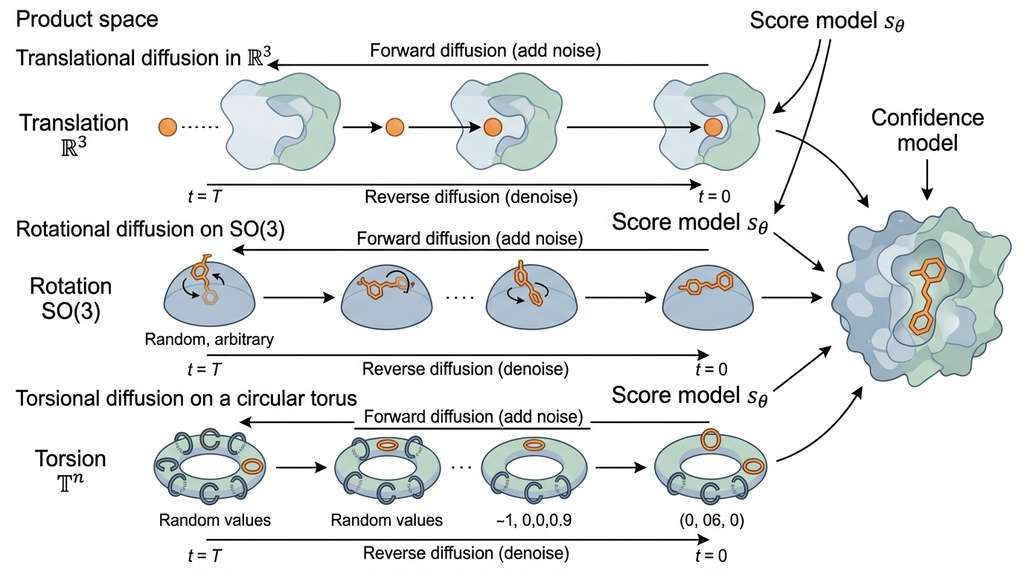
The key insight is that a ligand pose can be parameterized by three groups of degrees of freedom: (1) translation \(\mathbf{t} \in \mathbb{R}^3\), the position of the ligand center of mass relative to the protein; (2) rotation \(\mathbf{R} \in SO(3)\), where \(SO(3)\) is the group of all 3D rotations, representing the overall orientation of the ligand; and (3) torsion angles \(\boldsymbol{\tau} \in [0, 2\pi)^{n_{\text{tor}}}\), the rotatable bond angles that determine the ligand conformation. DiffDock defines a diffusion process on the product space \(\mathbb{R}^3 \times SO(3) \times \mathbb{T}^{n_{\text{tor}}}\):
$$q(\mathbf{t}_t, \mathbf{R}_t, \boldsymbol{\tau}_t | \mathbf{t}_0, \mathbf{R}_0, \boldsymbol{\tau}_0) = p_{\text{tr}}(\mathbf{t}_t | \mathbf{t}_0, t) \cdot p_{\text{rot}}(\mathbf{R}_t | \mathbf{R}_0, t) \cdot p_{\text{tor}}(\boldsymbol{\tau}_t | \boldsymbol{\tau}_0, t)$$The translational component uses standard Gaussian diffusion. The rotational component uses the isotropic Gaussian distribution on \(SO(3)\) (the IGSO(3) distribution), which has a closed-form density in terms of the rotation angle. The torsional component uses a wrapped normal distribution on the torus (torsion angles are periodic, wrapping from \(2\pi\) back to \(0\), so they live on a circle; with \(n_{\text{tor}}\) such angles, the space is a product of circles, forming a torus \(\mathbb{T}^{n_{\text{tor}}}\)). Note that the word "score" in this diffusion context means the gradient of the log-probability density, \(\nabla \log p\), which guides the denoising direction; this is unrelated to the "scoring function" of classical docking discussed above. The reverse diffusion process learns to denoise from random poses back to the crystal pose, using a score model \(\mathbf{s}_\theta\) that predicts the score in each component of the product space. Figure 49.2.1 illustrates DiffDock diffusion-based docking on the product space of translation, rotation, and torsion angles.
Checkpoint
So far: DiffDock parameterizes a ligand pose as a point in a combined translation, rotation, and torsion space, defines a forward diffusion that corrupts each component with appropriate noise, and trains a score model that learns to reverse this corruption, denoising random poses back toward the true binding pose.
Mental Model
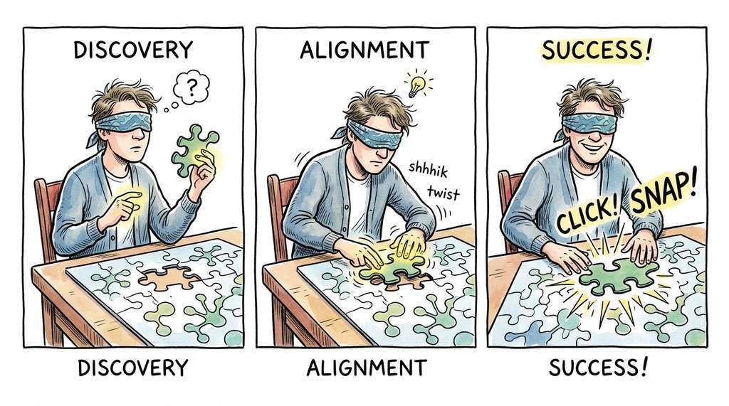
Think of DiffDock's diffusion process like reassembling a jigsaw puzzle piece into its slot while blindfolded. Imagine someone takes a puzzle piece (the ligand), tosses it randomly onto the table (forward diffusion adds noise to position, orientation, and shape), and then you must guide it back into its correct slot (the binding pocket) using only touch. At each step you feel how well the piece fits and nudge it: slide it a little (translation), twist it (rotation), and flex its tabs (torsion angles). Each nudge is small and informed by local fit, gradually refining from a random placement to the correct pose. The three types of adjustment (sliding, twisting, flexing) correspond exactly to the three components of DiffDock's product space, and the "feel" at each step is the learned score function telling the model which direction improves the fit.
After generating multiple pose hypotheses (typically 40), DiffDock ranks them with a learned confidence model that predicts the root-mean-square deviation (RMSD) of each generated pose relative to the (unknown) true pose. The confidence model is trained on the same crystal structure data, using the actual RMSD as supervision.
import subprocess
import json
from pathlib import Path
from dataclasses import dataclass


@dataclass
class DockingResult:
    """Result from a DiffDock docking run."""
    ligand_smiles: str
    protein_pdb: str
    pose_sdf: str          # Path to predicted pose SDF
    confidence: float      # Learned confidence score
    rank: int              # Rank among generated poses


def run_diffdock(
    protein_pdb: str,
    ligand_smiles: str,
    output_dir: str,
    n_poses: int = 40,
    diffdock_dir: str = "DiffDock",
) -> list[DockingResult]:
    """Run DiffDock to predict ligand binding poses.

    Args:
        protein_pdb: Path to protein PDB file.
        ligand_smiles: SMILES string of the ligand.
        output_dir: Directory for output poses.
        n_poses: Number of poses to generate.
        diffdock_dir: Path to DiffDock installation.

    Returns:
        List of DockingResult sorted by confidence (best first).
    """
    out = Path(output_dir)
    out.mkdir(parents=True, exist_ok=True)

    # Write input CSV for DiffDock
    csv_path = out / "input.csv"
    csv_path.write_text(
        "complex_name,protein_path,ligand_description,protein_sequence\n"
        f"complex_0,{protein_pdb},{ligand_smiles},\n"
    )

    # Run DiffDock inference
    cmd = [
        "python", f"{diffdock_dir}/inference.py",
        "--config", f"{diffdock_dir}/default_inference_args.yaml",
        "--protein_ligand_csv", str(csv_path),
        "--out_dir", str(out),
        "--samples_per_complex", str(n_poses),
        "--batch_size", "10",
        "--actual_steps", "18",
        "--no_final_step_noise",
    ]
    subprocess.run(cmd, check=True, capture_output=True)

    # Parse results: DiffDock outputs ranked SDF files
    results = []
    complex_dir = out / "complex_0"
    for sdf_path in sorted(complex_dir.glob("rank*.sdf")):
        rank = int(sdf_path.stem.replace("rank", "").split("_")[0])
        # Confidence is stored in the SDF file properties
        confidence = _parse_confidence(sdf_path)
        results.append(DockingResult(
            ligand_smiles=ligand_smiles,
            protein_pdb=protein_pdb,
            pose_sdf=str(sdf_path),
            confidence=confidence,
            rank=rank,
        ))

    return sorted(results, key=lambda r: -r.confidence)


def _parse_confidence(sdf_path: Path) -> float:
    """Extract confidence score from DiffDock SDF output."""
    text = sdf_path.read_text()
    for line in text.split("\n"):
        if "confidence" in line.lower():
            try:
                return float(line.strip())
            except ValueError:
                continue
    return 0.0
3. Boltz-1: Open-Source Biomolecular Cofolding
DiffDock generates high-quality poses, but it still requires a pre-determined protein structure as input, leaving it unable to capture the conformational changes that many targets undergo upon ligand binding. Boltz-1 removes that limitation by predicting the protein and ligand structures jointly.
Boltz-1 (Wohlwend et al., 2024) extends the AlphaFold paradigm from single-chain protein folding to general biomolecular complex prediction. (As of 2025, Boltz-2 adds property prediction heads for binding affinity and confidence-calibrated pocket detection on top of the original structure prediction architecture, narrowing the gap with AlphaFold 3 on protein-ligand benchmarks.) Given a protein sequence and a ligand (specified as SMILES, Chemical Component Dictionary (CCD) code, or a molecular graph), Boltz-1 predicts the 3D structure of the entire complex, including both the protein conformation and the ligand binding pose.
The architecture combines ideas from AlphaFold2 and RoseTTAFold-AllAtom. Multiple Sequence Alignments (MSAs), where each alignment collects evolutionarily related sequences to reveal conserved residues, provide evolutionary context for the protein. The ligand is represented as a molecular graph with atom-level features. A trunk module processes paired representations of protein residues and ligand atoms through alternating self-attention and cross-attention layers. A structure module then converts these representations into 3D coordinates, using an iterative refinement process similar to AlphaFold2's structure module.
Boltz-1 outputs per-residue and per-atom confidence scores (analogous to AlphaFold2's predicted Local Distance Difference Test (pLDDT)), plus an interface predicted Template Modeling score (ipTM) that specifically measures the reliability of the protein-ligand interface prediction. Based on the authors' published validation, an ipTM above 0.7 typically indicates a reliable binding mode prediction; below 0.5 suggests the model is uncertain about the interaction.
Common Misconception
A frequent mistake is treating the cofolding confidence score (ipTM) as a proxy for binding affinity. High ipTM means the model is confident about the predicted geometry of the complex (the pose is likely correct), not that the ligand binds tightly. A molecule can sit in the pocket with a geometrically precise pose (ipTM = 0.9) yet bind weakly because the interaction lacks favorable enthalpic contacts or pays a large desolvation penalty (the energetic cost of stripping away solvent molecules that were surrounding the ligand and the binding pocket before they came together). Binding affinity requires separate estimation (Section 5 below); ipTM tells you whether to trust the predicted structure, not whether the compound is a good drug.
import subprocess
import json
from pathlib import Path
from dataclasses import dataclass, field
import numpy as np


@dataclass
class CofoldingResult:
    """Result from a Boltz-1 cofolding prediction."""
    protein_sequence: str
    ligand_smiles: str
    complex_pdb: str       # Path to predicted complex PDB
    plddt_mean: float      # Mean per-residue confidence
    iptm: float            # Interface predicted TM-score
    ligand_coords: np.ndarray = field(repr=False)  # (n_atoms, 3)


def run_boltz1(
    protein_fasta: str,
    ligand_smiles: str,
    output_dir: str,
    n_recycling: int = 3,
    n_samples: int = 5,
) -> list[CofoldingResult]:
    """Run Boltz-1 cofolding prediction.

    Predicts the 3D structure of a protein-ligand complex,
    including protein conformation and ligand binding pose.

    Args:
        protein_fasta: Path to protein FASTA file.
        ligand_smiles: SMILES string of the ligand.
        output_dir: Directory for output structures.
        n_recycling: Number of recycling iterations.
        n_samples: Number of structure samples to generate.

    Returns:
        List of CofoldingResult sorted by ipTM (best first).
    """
    out = Path(output_dir)
    out.mkdir(parents=True, exist_ok=True)

    # Write Boltz-1 input YAML
    input_yaml = out / "input.yaml"
    input_yaml.write_text(f"""
sequences:
  - protein:
      id: A
      fasta_file: {protein_fasta}
  - ligand:
      id: B
      smiles: "{ligand_smiles}"
""")

    # Run Boltz-1 inference
    cmd = [
        "boltz", "predict",
        str(input_yaml),
        "--out_dir", str(out),
        "--recycling_steps", str(n_recycling),
        "--num_samples", str(n_samples),
        "--use_msa_server",
    ]
    subprocess.run(cmd, check=True, capture_output=True)

    # Parse results
    results = []
    for pdb_path in sorted(out.glob("predictions/*.pdb")):
        confidence = _parse_boltz_confidence(
            out / "predictions" / "confidence.json",
            pdb_path.stem,
        )
        ligand_coords = _extract_ligand_coords(pdb_path, chain_id="B")

        # Read protein sequence from FASTA
        protein_seq = Path(protein_fasta).read_text().split("\n", 1)[1].replace("\n", "")

        results.append(CofoldingResult(
            protein_sequence=protein_seq,
            ligand_smiles=ligand_smiles,
            complex_pdb=str(pdb_path),
            plddt_mean=confidence.get("plddt_mean", 0.0),
            iptm=confidence.get("iptm", 0.0),
            ligand_coords=ligand_coords,
        ))

    return sorted(results, key=lambda r: -r.iptm)


def _parse_boltz_confidence(json_path: Path, model_name: str) -> dict:
    """Parse Boltz-1 confidence metrics from JSON output."""
    if not json_path.exists():
        return {}
    data = json.loads(json_path.read_text())
    return data.get(model_name, {})


def _extract_ligand_coords(pdb_path: Path, chain_id: str) -> np.ndarray:
    """Extract ligand atom coordinates from a PDB file."""
    coords = []
    for line in pdb_path.read_text().split("\n"):
        if line.startswith(("HETATM", "ATOM")) and line[21] == chain_id:
            x = float(line[30:38])
            y = float(line[38:46])
            z = float(line[46:54])
            coords.append([x, y, z])
    return np.array(coords) if coords else np.empty((0, 3))
4. Chai-1: Multi-Modal Molecular Structure Prediction
Chai-1 (Chai Discovery, 2024) takes the cofolding concept further by handling arbitrary combinations of biomolecular entities: proteins, small molecules, DNA, RNA, ions, and covalent modifications. Where Boltz-1 focuses on protein-ligand pairs, Chai-1 can predict the structure of a ternary complex (e.g., a protein bound to both a DNA strand and a small molecule cofactor) in a single forward pass.
Chai-1's architecture uses a multi-track Transformer that processes each entity type with specialized tokenization but shares attention across tracks. Proteins are tokenized at the residue level, nucleic acids at the nucleotide level, and small molecules at the atom level. Cross-track attention allows the model to learn how each entity type influences the conformation of the others.
Chai-1's chief advantage over Boltz-1 for drug discovery is its handling of cofactors and metal ions. Many drug targets are metalloenzymes or require cofactors (NAD+, FAD, ATP) for function; ignoring these entities mispredicts binding site geometry and degrades pose accuracy. Chai-1's multi-modal architecture accommodates them through its shared cross-track attention, requiring no entity-specific workarounds.
import torch
from chai_lab.chai1 import run_inference


def predict_complex_chai1(
    fasta_path: str,
    ligand_smiles: str,
    output_dir: str,
    num_trunk_recycles: int = 3,
    num_diffn_timesteps: int = 200,
    device: str = "cuda",
) -> dict:
    """Predict a protein-ligand complex structure using Chai-1.

    Chai-1 handles proteins, ligands, nucleic acids, and ions
    in a unified multi-modal framework.

    Args:
        fasta_path: Path to multi-entity FASTA file.
        ligand_smiles: Ligand SMILES (can also be CCD code).
        output_dir: Directory for output structures.
        num_trunk_recycles: Trunk recycling iterations.
        num_diffn_timesteps: Diffusion timesteps for structure module.
        device: Compute device.

    Returns:
        Dict with predicted structure path and confidence scores.
    """
    # Chai-1 expects a specially formatted FASTA with entity tags
    # >protein|name=kinase
    # MVLSPADKTN...
    # >ligand|name=inhibitor
    # CC(=O)Nc1ccc(O)cc1

    candidates = run_inference(
        fasta_file=fasta_path,
        output_dir=output_dir,
        num_trunk_recycles=num_trunk_recycles,
        num_diffn_timesteps=num_diffn_timesteps,
        seed=42,
        device=torch.device(device),
        use_esm_embeddings=True,
    )

    # candidates is a list of SampleOutput objects
    best = max(candidates.samples, key=lambda s: s.aggregate_score)

    return {
        "pdb_path": best.pdb_path,
        "aggregate_score": float(best.aggregate_score),
        "ptm": float(best.ptm),
        "iptm": float(best.iptm),
        "per_chain_ptm": {
            chain: float(score)
            for chain, score in best.per_chain_ptm.items()
        },
        "clash_score": float(best.clash_score),
        "ranking_score": float(best.ranking_score),
    }


# Example: predict kinase-inhibitor complex
result = predict_complex_chai1(
    fasta_path="data/kinase_complex.fasta",
    ligand_smiles="CC(=O)Nc1ccc(F)c(Nc2nccc(-c3cccnc3)n2)c1",
    output_dir="outputs/chai1_kinase/",
)
print(f"ipTM: {result['iptm']:.3f}, "
      f"Aggregate: {result['aggregate_score']:.3f}")
A biotech company wants to find inhibitors for a metalloenzyme target that has no known crystal structure with a bound ligand. They have the apo crystal structure and a library of 10,000 candidate compounds. Traditional docking against the apo structure performs poorly because the binding site rearranges upon ligand binding.
Their computational pipeline uses Chai-1 to predict the holo structure for each compound, accounting for induced fit. Because Chai-1 inference takes roughly 2 minutes per complex on an A100 GPU, processing 10,000 compounds requires approximately 330 GPU-hours. They filter the library first using 2D similarity to known metalloenzyme inhibitors (keeping 2,000 candidates), then run Chai-1 on this focused set. Compounds are ranked by ipTM score, and the top 100 (ipTM > 0.75) are inspected manually. Twenty compounds are purchased and tested in a biochemical assay, yielding four confirmed hits (20% hit rate), compared to an often-cited industry estimate of 1-2% hit rate from traditional high-throughput screening (HTS), though actual HTS hit rates vary widely by target and assay format.
5. Binding Affinity Estimation
The cofolding models above tell us where a ligand sits in the binding pocket, but a drug candidate must also bind tightly enough to be therapeutically useful, and that requires a separate estimation step.
Cofolding models predict structure, not affinity. Knowing that a ligand binds in a particular pose does not tell you how tightly it binds. The binding free energy \(\Delta G_{\text{bind}}\) determines the equilibrium dissociation constant \(K_d\) (the ligand concentration at which half the protein molecules are bound) through the fundamental thermodynamic relationship:
$$\Delta G_{\text{bind}} = RT \ln K_d$$where \(R\) is the gas constant and \(T\) is the temperature. A difference of just 1.4 kcal/mol in \(\Delta G\) corresponds to a 10-fold change in \(K_d\) at room temperature. Predicting \(\Delta G\) to within 1 kcal/mol (the threshold for useful rank-ordering of compounds) remains one of the hardest unsolved problems in computational chemistry.
Three approaches follow cofolding. Physics-based rescoring applies molecular mechanics force fields (Molecular Mechanics Generalized Born Surface Area (MM-GBSA), Molecular Mechanics Poisson-Boltzmann Surface Area (MM-PBSA)) to the predicted complex, computing van der Waals, electrostatic, and solvation energies. This approach is principled but slow and only moderately accurate. Learned scoring functions train neural networks to predict \(\Delta G\) from complex features (interatomic distances, hydrogen bonds, hydrophobic contacts). They run fast but tend to learn dataset biases rather than physics. Relative free energy perturbation (FEP) uses molecular dynamics simulations to compute the difference in binding free energy between pairs of similar compounds. In favorable cases, FEP achieves among the highest accuracy available (typically around 1 kcal/mol for congeneric series, where a congeneric series is a set of compounds sharing the same core scaffold but differing by small chemical substituents) but requires hours of GPU time per compound pair.
import numpy as np
from scipy.spatial.distance import cdist


def interaction_fingerprint(
    protein_coords: np.ndarray,
    protein_elements: list[str],
    ligand_coords: np.ndarray,
    ligand_elements: list[str],
    distance_bins: tuple = (2.0, 3.0, 4.0, 5.0, 6.0),
) -> np.ndarray:
    """Compute a protein-ligand interaction fingerprint.

    Encodes the pattern of contacts between protein and ligand
    atoms at multiple distance thresholds, stratified by atom type
    pairs. Used as input features for learned scoring functions.

    Args:
        protein_coords: (n_prot, 3) protein atom positions.
        protein_elements: List of protein atom element symbols.
        ligand_coords: (n_lig, 3) ligand atom positions.
        ligand_elements: List of ligand atom element symbols.
        distance_bins: Distance thresholds in Angstroms.

    Returns:
        1D fingerprint vector encoding interaction pattern.
    """
    # Compute all pairwise distances
    dist_matrix = cdist(protein_coords, ligand_coords)

    # Define atom type groups
    type_map = {
        "C": "hydrophobic", "S": "hydrophobic",
        "N": "donor_acceptor", "O": "donor_acceptor",
        "F": "halogen", "Cl": "halogen", "Br": "halogen",
    }
    prot_types = [type_map.get(e, "other") for e in protein_elements]
    lig_types = [type_map.get(e, "other") for e in ligand_elements]

    # Enumerate interaction type pairs
    type_names = ["hydrophobic", "donor_acceptor", "halogen", "other"]
    pair_names = []
    for pt in type_names:
        for lt in type_names:
            pair_names.append(f"{pt}-{lt}")

    # Count contacts at each distance threshold for each type pair
    fingerprint = []
    for bin_dist in distance_bins:
        contacts = dist_matrix < bin_dist
        for pt in type_names:
            for lt in type_names:
                prot_mask = np.array([t == pt for t in prot_types])
                lig_mask = np.array([t == lt for t in lig_types])
                count = contacts[np.ix_(prot_mask, lig_mask)].sum()
                fingerprint.append(count)

    return np.array(fingerprint, dtype=np.float32)


# Example: compute fingerprint for a predicted complex
# prot_coords, prot_elem = parse_protein("complex.pdb")
# lig_coords, lig_elem = parse_ligand("complex.pdb")
# fp = interaction_fingerprint(prot_coords, prot_elem,
#                              lig_coords, lig_elem)
# affinity = scoring_model.predict(fp.reshape(1, -1))
The interaction fingerprint above is a simplified version of what the ProLIF library (Protein-Ligand Interaction Fingerprints) computes automatically. ProLIF detects hydrogen bonds, salt bridges, pi-stacking, hydrophobic contacts, and metal coordination from a single function call, reducing the 50-line implementation to three lines. It integrates directly with MDAnalysis for trajectory analysis and with RDKit for molecular manipulation.
import prolif
import MDAnalysis as mda

u = mda.Universe("complex.pdb")
prot = u.select_atoms("protein")
lig = u.select_atoms("resname LIG")
fp = prolif.Fingerprint()
fp.run(u.trajectory, lig, prot)
df = fp.to_dataframe()  # Interaction matrix across frames
6. Building a Cofolding Pipeline with Confidence Filtering
A practical cofolding pipeline must handle failures gracefully. Not every protein-ligand pair will produce a reliable prediction. The pipeline below runs Boltz-1 on a batch of candidates, filters by confidence, and produces a ranked list suitable for experimental follow-up or further computational refinement.
from dataclasses import dataclass
from pathlib import Path
import json
import logging

logger = logging.getLogger(__name__)


@dataclass
class CofoldCandidate:
    """A ligand candidate with cofolding results."""
    smiles: str
    name: str
    iptm: float
    plddt_mean: float
    complex_pdb: str
    passed_filter: bool


def cofolding_pipeline(
    protein_fasta: str,
    ligands: list[dict],          # [{"smiles": ..., "name": ...}, ...]
    output_dir: str,
    iptm_threshold: float = 0.65,
    plddt_threshold: float = 60.0,
    max_clashes: int = 5,
) -> list[CofoldCandidate]:
    """Run a cofolding screen with confidence-based filtering.

    Args:
        protein_fasta: Path to target protein FASTA.
        ligands: List of ligand dicts with 'smiles' and 'name'.
        output_dir: Base output directory.
        iptm_threshold: Minimum ipTM for passing.
        plddt_threshold: Minimum mean pLDDT for passing.
        max_clashes: Maximum allowed atomic clashes.

    Returns:
        Sorted list of CofoldCandidate (best ipTM first).
    """
    out = Path(output_dir)
    results = []

    for i, lig in enumerate(ligands):
        lig_dir = out / f"ligand_{i:04d}"
        logger.info(f"Cofolding {lig['name']} ({i+1}/{len(ligands)})")

        try:
            cofold_results = run_boltz1(
                protein_fasta=protein_fasta,
                ligand_smiles=lig["smiles"],
                output_dir=str(lig_dir),
                n_samples=3,
            )

            if not cofold_results:
                logger.warning(f"No results for {lig['name']}")
                continue

            best = cofold_results[0]  # Highest ipTM

            # Apply confidence filters
            passed = (
                best.iptm >= iptm_threshold
                and best.plddt_mean >= plddt_threshold
            )

            results.append(CofoldCandidate(
                smiles=lig["smiles"],
                name=lig["name"],
                iptm=best.iptm,
                plddt_mean=best.plddt_mean,
                complex_pdb=best.complex_pdb,
                passed_filter=passed,
            ))

        except Exception as e:
            logger.error(f"Failed for {lig['name']}: {e}")
            continue

    # Sort by ipTM descending
    results.sort(key=lambda r: -r.iptm)

    # Summary statistics
    n_passed = sum(1 for r in results if r.passed_filter)
    logger.info(
        f"Cofolding complete: {len(results)}/{len(ligands)} succeeded, "
        f"{n_passed} passed filters (ipTM>={iptm_threshold}, "
        f"pLDDT>={plddt_threshold})"
    )

    # Save results summary
    summary = [
        {
            "name": r.name, "smiles": r.smiles,
            "iptm": r.iptm, "plddt": r.plddt_mean,
            "passed": r.passed_filter, "pdb": r.complex_pdb,
        }
        for r in results
    ]
    (out / "cofolding_summary.json").write_text(
        json.dumps(summary, indent=2)
    )

    return results
Research Frontier
AlphaFold 3 (Abramson et al., 2024, Nature) represents the current frontier in biomolecular structure prediction. Unlike AlphaFold2, which predicted only protein structures, AlphaFold 3 uses a diffusion-based architecture to jointly predict complexes of proteins, nucleic acids, small molecules, ions, and covalent modifications within a single unified model. On the PoseBusters benchmark for protein-ligand docking, AlphaFold 3 achieves state-of-the-art accuracy, surpassing both DiffDock and specialized docking tools on realistic drug-like molecules. Its structure module replaces the Evoformer's direct coordinate output with an iterative diffusion process that denoises atom positions (the Evoformer is AlphaFold2's core attention module that processes MSA and pairwise representations into structural features), enabling it to handle the diversity of chemical entities without entity-specific architecture branches. As of mid-2025, AlphaFold 3 is accessible through the AlphaFold Server for non-commercial use and through Google Cloud for commercial applications, though open-weight alternatives (Boltz-1, Chai-1, OpenFold3) continue to close the accuracy gap.
Try It: Visualize a Predicted Protein-Ligand Complex
Build a mini-pipeline that fetches a protein structure, docks a known drug, and visualizes the result, all on a standard laptop with no GPU required.
Step 1. Install dependencies: pip install biopython rdkit-pypi py3Dmol requests numpy.
Step 2. Download a protein structure from the PDB. Use BioPython to fetch human carbonic anhydrase II (PDB ID: 2WEJ), which contains a co-crystallized sulfonamide inhibitor: from Bio.PDB import PDBList; PDBList().retrieve_pdb_file("2WEJ", pdir=".", file_format="pdb").
Step 3. Extract the ligand and protein separately. Parse the PDB file, write all ATOM records (protein) to protein_only.pdb and all HETATM records for the ligand residue (residue name "VIB") to ligand_only.pdb. Exclude water molecules (HOH).
Step 4. Compute a basic interaction fingerprint. Using the interaction_fingerprint function from this section (or SciPy's cdist), calculate all protein-ligand atom distances and count the number of close contacts (below 4 Angstroms) stratified by element type. Print which atom-type pairs contribute the most contacts.
Step 5. Visualize the complex interactively. Use py3Dmol in a Jupyter notebook: import py3Dmol; view = py3Dmol.view(); view.addModel(open("pdb2wej.ent").read(), "pdb"); view.setStyle({"chain": "A"}, {"cartoon": {"color": "spectrum"}}); view.setStyle({"resn": "VIB"}, {"stick": {"colorscheme": "greenCarbon"}}); view.zoomTo({"resn": "VIB"}); view.show(). Rotate the view to identify the binding pocket residues surrounding the ligand. Compare what you see with the contact analysis from Step 4.
Exercise 49.2.1
A cofolding model predicts five poses for a ligand with ipTM scores of 0.82, 0.74, 0.68, 0.55, and 0.41, and corresponding mean pLDDT values of 78, 72, 65, 58, and 50. You apply a confidence filter requiring ipTM ≥ 0.65 and pLDDT ≥ 60. (a) Which poses pass the filter? (b) The experimental crystal structure reveals that pose 3 (ipTM = 0.68) has the lowest ligand RMSD to the true binding mode. Does this pose survive your filter? (c) If the ipTM threshold were raised to 0.75, how many poses would remain, and what risk does a stricter threshold introduce for a virtual screening campaign?
Hint
Apply both thresholds jointly: a pose must satisfy both criteria to pass. For part (c), consider that stricter thresholds reduce false positives but increase false negatives, potentially discarding genuine binders whose predicted geometry is slightly less confident.
Step-Through: DiffDock Reverse Diffusion on a 2D Toy Example
Trace through DiffDock's reverse diffusion with a simplified 2D analogy. Suppose the true ligand pose has translation \((3.0, 5.0)\), rotation \(\theta = 45°\), and one torsion angle \(\tau = 120°\).
t = T (fully noised): The sampled starting state is translation \((8.2, 1.7)\), rotation \(\theta = 263°\), torsion \(\tau = 37°\). The ligand is far from the binding pocket, randomly oriented, and in a wrong conformation.
t = 0.75T: The score model predicts gradients: \(\nabla_t = (-1.8, +1.1)\), \(\nabla_\theta = -55°\), \(\nabla_\tau = +22°\). After the update step: translation \((6.4, 2.8)\), rotation \(\theta = 208°\), torsion \(\tau = 59°\). The ligand has drifted toward the pocket.
t = 0.50T: Score gradients: \(\nabla_t = (-1.5, +1.0)\), \(\nabla_\theta = -72°\), \(\nabla_\tau = +28°\). Updated state: translation \((4.9, 3.8)\), rotation \(\theta = 136°\), torsion \(\tau = 87°\). The ligand is approaching the correct region.
t = 0.25T: Score gradients: \(\nabla_t = (-1.1, +0.7)\), \(\nabla_\theta = -58°\), \(\nabla_\tau = +20°\). Updated state: translation \((3.8, 4.5)\), rotation \(\theta = 78°\), torsion \(\tau = 107°\). Pose is close to the crystal pose.
t = 0 (final): Score gradients: \(\nabla_t = (-0.8, +0.5)\), \(\nabla_\theta = -33°\), \(\nabla_\tau = +13°\). Final state: translation \((3.0, 5.0)\), rotation \(\theta = 45°\), torsion \(\tau = 120°\). The ligand has converged to the true binding pose. Notice how the step sizes shrink as the model gains confidence near the solution, a hallmark of the diffusion denoising schedule.
Real-World Application: PROTAC Design at Arvinas
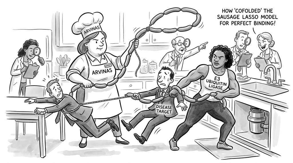
Arvinas, a clinical-stage biotech company, uses cofolding models to design PROTACs (proteolysis-targeting chimeras), bifunctional molecules that simultaneously bind a disease target and an E3 ubiquitin ligase to induce targeted protein degradation. Predicting the ternary complex (target protein, PROTAC linker, E3 ligase) requires modeling two protein-ligand interfaces and the geometry of the linker connecting them. Chai-1's multi-entity cofolding capability allows Arvinas to evaluate whether a given linker length and geometry can bridge the two proteins in a productive orientation, reducing the design cycle from months of trial-and-error synthesis to days of computational screening.
The Billion-Dollar Blind Spot
In 2023, researchers at MIT benchmarked leading docking and cofolding tools on the PoseBusters dataset, which enforces basic chemical validity checks (correct bond lengths, no atom clashes, proper chirality). Several models that achieved impressive RMSD scores on standard benchmarks saw their success rates drop by 20% or more once chemically invalid poses were excluded. DiffDock, for instance, predicted poses that sometimes placed ligand atoms physically inside protein atoms or assigned bond geometries that violate basic valence rules. The lesson: a pose can look statistically close to the crystal structure (low RMSD) while being physically impossible. This discovery prompted every major cofolding group to add post-prediction validity filters, a humbling reminder that neural networks can learn to match coordinates without learning chemistry.
Lab: Compare Docking and Cofolding on a Known Complex
Goal: Dock a known inhibitor into its target using both a classical docking tool and a cofolding model, then compare the predicted poses against the experimental crystal structure.
Tools needed: Python 3.9+, pip install meeko vina biopython rdkit-pypi numpy scipy. For cofolding, use the Boltz-1 web server (boltz.mit.edu) or install Boltz-1 locally if a GPU is available.
Protocol (25 min): (1) Download PDB 3HTB (CDK2 with a bound inhibitor, residue name DTQ). Extract the protein and ligand separately. (2) Run AutoDock Vina: prepare the receptor with meeko, define a search box centered on the ligand's center of mass with a 20 Angstrom side length, and dock. Record the top-5 pose RMSDs against the crystal ligand coordinates. (3) Submit the CDK2 sequence and DTQ SMILES to the Boltz-1 server. Download the predicted complex and compute the ligand RMSD. (4) Compare: which method places more atoms within 2 Angstroms of their crystal positions? Which method better captures the orientation of the inhibitor's aromatic rings?
What to vary: Try removing the co-crystallized water molecules before docking (they often mediate key contacts). Try a second ligand (e.g., PDB 1H1Q, same target, different inhibitor scaffold) and observe whether the accuracy gap between methods changes.
What to observe: Classical docking typically finds reasonable poses for well-defined pockets but struggles with induced-fit rearrangements. Cofolding models may capture backbone shifts but can introduce physically implausible bond geometries. Check both RMSD and chemical validity (bond lengths, atom clashes) to get a complete picture.
What's Next
Molecular generation and cofolding address the "soft matter" side of chemistry: organic molecules interacting with biological macromolecules. The next section, Section 49.3: Materials Design and Universal Force Fields, turns to the "hard matter" side: crystalline materials, inorganic compounds, and the machine-learned interatomic potentials that make it possible to simulate materials across the entire periodic table without running expensive quantum mechanical calculations for each new system.