"I computed the exact probability of every possible next reaction. Then I rolled a die. People think stochastic simulation is random. It is the opposite: it is randomness done correctly."
A Propensity Function With Standards
When molecules number in the hundreds rather than the billions, the smooth curves of ordinary differential equations lie. A cell with 50 copies of a transcription factor does not experience continuous concentration changes; it experiences discrete, stochastic events: one molecule binds, another degrades, a burst of mRNA appears. The Gillespie algorithm simulates these events exactly, producing sample paths that honor the underlying probability theory. At a different scale, molecular dynamics tracks every atom in a protein as it vibrates, folds, and interacts with water, solving Newton's equations at femtosecond resolution. This section covers both regimes: chemical kinetics at the stochastic level and atomic physics at the molecular level.
1. The Gillespie Algorithm
A living cell carries just ten copies of a critical transcription factor, and in the next millisecond one of them will either bind its target gene or get shredded by a protease; which event happens first determines whether the cell divides or stays dormant, and no smooth differential equation can tell you the answer. The Stochastic Simulation Algorithm (SSA), published by Daniel Gillespie in 1977, was built for exactly this regime: simulating the time evolution of a well-stirred chemical system when molecule counts are small enough that stochastic fluctuations control the outcome.
What. The Gillespie algorithm produces exact sample paths of the Chemical Master Equation (CME), where the CME is the probability distribution over all possible states of a reaction system describing how that distribution evolves in time. Each sample path is a sequence of discrete reaction events, with both the time of the next event and the identity of the next reaction determined by the current state.
Why. Deterministic rate equations, typically ordinary differential equations (ODEs), describe the mean behavior of a system in the limit of infinite molecules. For systems with low copy numbers (gene regulatory networks, single-cell biology, early-stage viral infection), the mean is a poor summary. Stochastic fluctuations drive phenomena like bistability, noise-induced switching, and stochastic focusing that deterministic models miss entirely.
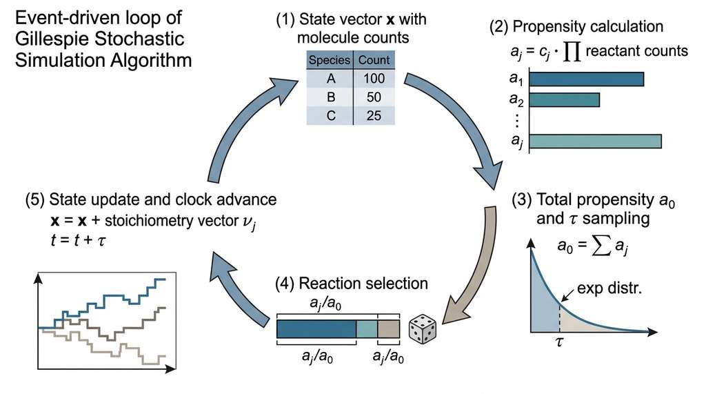
How. The algorithm maintains a state vector \(\mathbf{x} = (x_1, x_2, \ldots, x_N)\) counting the molecules of each species. Figure 43.2 illustrates the iterative loop. At each step:
- Compute the propensity \(a_j(\mathbf{x})\) of each reaction \(j\). For a unimolecular reaction \(A \to B\) with rate constant \(c_j\), the propensity is \(a_j = c_j \cdot x_A\). For a bimolecular reaction \(A + B \to C\), it is \(a_j = c_j \cdot x_A \cdot x_B\).
- Compute the total propensity \(a_0 = \sum_j a_j\).
- Draw the time to the next event from an exponential distribution: \(\tau \sim \text{Exp}(a_0)\).
- Choose which reaction fires with probability proportional to its propensity: \(P(\text{reaction } j) = a_j / a_0\).
- Update the state vector and the clock: \(\mathbf{x} \leftarrow \mathbf{x} + \boldsymbol{\nu}_j\), \(t \leftarrow t + \tau\), where \(\boldsymbol{\nu}_j\) is the stoichiometry vector (the net change in each species count) for reaction \(j\).
The beauty of the algorithm is that steps 3 and 4 are exact: no approximation, no discretization error. The sample path is a draw from the true probability distribution over trajectories. In short: the Gillespie algorithm does not add randomness to a model; it faithfully simulates the randomness that is already there. Figure 43.2.1 illustrates Gillespie algorithm event-driven simulation loop.
Mental Model

Think of the Gillespie algorithm like a kitchen with several dishes cooking on different burners. Each dish (reaction) has its own timer, but the timers are not set to fixed intervals; instead, each timer rings sooner when the dish needs more frequent stirring (higher propensity). You always attend to whichever timer rings first, stir that dish, then all the timers reset based on the new state of the kitchen. If one pot boils down (reactant is consumed), its timer slows; if another pot starts bubbling over (product accumulates), its timer speeds up. You never need to check every burner at once; the timers tell you exactly when and where to act next. This is why the algorithm is both event-driven and exact: it lets the system's own dynamics schedule every intervention.
The propensity \(a_j(\mathbf{x})\) is the probability per unit time that reaction \(j\) fires in state \(\mathbf{x}\). It depends on both the rate constant \(c_j\) and the current molecule counts. This state-dependence is what makes the Gillespie algorithm faithful to the underlying physics: as reactants are consumed, the propensity drops; as products accumulate and become reactants for downstream reactions, new propensities rise. The system's dynamics emerge from this interplay, not from a fixed set of rates.
Common Misconception
A frequent mistake is believing that stochastic simulation produces "noisy" or "unreliable" results compared to deterministic ODE models, and that running enough replicates would converge to the ODE solution. This is wrong: the stochasticity is not numerical noise to be averaged away; it is a physical property of the system. When molecule counts are small, the probability distribution over states is broad and often multimodal (for example, a gene regulatory switch can be in an "on" or "off" state, with the ODE solution landing at an unphysical average between the two). The Gillespie algorithm samples from the true distribution; the ODE gives only the mean of that distribution, which may correspond to no physically realizable state at all.
1.1 Implementing the Gillespie Algorithm
The Lotka-Volterra predator-prey model exhibits the oscillatory dynamics that make stochastic effects most visible.
$$ \begin{align} R_1: &\quad \text{Prey} \xrightarrow{c_1} 2\,\text{Prey} \quad &\text{(prey reproduction)} \\ R_2: &\quad \text{Prey} + \text{Predator} \xrightarrow{c_2} 2\,\text{Predator} \quad &\text{(predation)} \\ R_3: &\quad \text{Predator} \xrightarrow{c_3} \emptyset \quad &\text{(predator death)} \end{align} $$import numpy as np
from dataclasses import dataclass
@dataclass
class Reaction:
"""A chemical reaction with reactant indices, stoichiometry, and rate."""
name: str
reactants: list # indices into species vector
stoichiometry: list # change in each species when reaction fires
rate_constant: float
def gillespie_ssa(species_init, reactions, t_max, seed=42):
"""Exact stochastic simulation using the Gillespie algorithm.
Args:
species_init: initial molecule counts, shape (n_species,)
reactions: list of Reaction objects
t_max: simulation end time
seed: random seed for reproducibility
Returns:
times: array of event times
states: array of shape (n_events, n_species)
"""
rng = np.random.default_rng(seed)
x = np.array(species_init, dtype=float)
t = 0.0
times = [t]
states = [x.copy()]
while t < t_max:
# Step 1: Compute propensities
propensities = np.zeros(len(reactions))
for j, rxn in enumerate(reactions):
prop = rxn.rate_constant
for idx in rxn.reactants:
prop *= x[idx]
propensities[j] = prop
a0 = propensities.sum()
if a0 == 0:
break # no reactions possible (extinction)
# Step 2: Time to next event
tau = rng.exponential(1.0 / a0)
t += tau
if t > t_max:
break
# Step 3: Which reaction fires?
j = rng.choice(len(reactions), p=propensities / a0)
# Step 4: Update state
x += reactions[j].stoichiometry
x = np.maximum(x, 0) # guard against numerical issues
times.append(t)
states.append(x.copy())
return np.array(times), np.array(states)
# Define the Lotka-Volterra system
reactions = [
Reaction("prey_birth", [0], [1, 0], 0.5), # Prey -> 2 Prey
Reaction("predation", [0, 1], [-1, 1], 0.005), # Prey + Pred -> 2 Pred
Reaction("predator_death", [1], [0, -1], 0.3), # Pred -> 0
]
times, states = gillespie_ssa(
species_init=[100, 50],
reactions=reactions,
t_max=50.0,
seed=42,
)
print(f"Simulation produced {len(times)} events over {times[-1]:.1f} time units")
print(f"Final state: Prey={states[-1, 0]:.0f}, Predators={states[-1, 1]:.0f}")Running multiple replications reveals the stochastic nature of the system. Some trajectories sustain oscillations indefinitely; others terminate in prey extinction (followed inevitably by predator extinction). The deterministic ODE model predicts perfect, eternal cycles. The stochastic model reveals that extinction is not only possible but, for many parameter regimes, probable over long time horizons, a qualitative difference that matters for conservation biology and epidemiology.
1.2 Tau-Leaping: Trading Exactness for Speed
The Gillespie algorithm is exact but slow: it processes one reaction at a time. For systems with thousands of molecules and fast reactions, the algorithm spends most of its time on events that barely change the state. Tau-leaping accelerates simulation by firing multiple reactions in a single time step.
Tau-leaping groups many reaction events into a single time step, approximating the exact Gillespie algorithm. It serves as the workhorse for chemical systems too large for event-by-event SSA but too small for deterministic ODEs. Exact SSA becomes intractable when systems contain thousands of molecules and hundreds of reaction channels, because each step processes only one event. Tau-leaping reduces the step count by two to three orders of magnitude. The method chooses a step size \(\tau\) small enough that no propensity changes beyond a specified tolerance during the interval. It then draws the number of firings of each reaction from independent Poisson distributions with means \(a_j(\mathbf{x}) \cdot \tau\). Use tau-leaping over exact SSA when molecule counts exceed roughly 100 and no extremely fast reactions force tiny \(\tau\). Fall back to exact SSA for very low copy numbers (under ~20 molecules), where the Poisson approximation breaks down. Switch to deterministic ODEs when counts exceed ~10,000 and stochastic effects become negligible.
The core mechanism: choose a time step \(\tau\) small enough that propensities do not change appreciably, then draw the number of times each reaction fires from a Poisson distribution:
$$k_j \sim \text{Poisson}(a_j(\mathbf{x}) \cdot \tau)$$def tau_leaping(species_init, reactions, t_max, tau=0.01, seed=42):
"""Approximate stochastic simulation using tau-leaping.
Fires multiple reactions per time step using Poisson-distributed
counts. Faster than exact SSA but introduces discretization error.
"""
rng = np.random.default_rng(seed)
x = np.array(species_init, dtype=float)
t = 0.0
times = [t]
states = [x.copy()]
while t < t_max:
propensities = np.zeros(len(reactions))
for j, rxn in enumerate(reactions):
prop = rxn.rate_constant
for idx in rxn.reactants:
prop *= x[idx]
propensities[j] = max(prop, 0)
if propensities.sum() == 0:
break
# Fire multiple reactions in one step
for j, rxn in enumerate(reactions):
if propensities[j] > 0:
n_firings = rng.poisson(propensities[j] * tau)
x += n_firings * np.array(rxn.stoichiometry)
x = np.maximum(x, 0)
t += tau
times.append(t)
states.append(x.copy())
return np.array(times), np.array(states)
times_tl, states_tl = tau_leaping(
species_init=[100, 50],
reactions=reactions,
t_max=50.0,
tau=0.01,
seed=42,
)
print(f"Tau-leaping: {len(times_tl)} steps (vs {len(times)} exact SSA events)")Tau-leaping can produce negative molecule counts when \(\tau\) is too large relative to the current populations. The np.maximum(x, 0) guard in the code above is a crude fix. Production implementations use adaptive tau selection (Cao et al., 2006) or the binomial tau-leap variant, which bounds the number of firings by the available reactant molecules. For discovery-oriented work where qualitative behavior matters more than exact counts, the simple guard suffices; for quantitative calibration, use adaptive methods or fall back to exact SSA.
2. Molecular Dynamics with OpenMM
Molecular dynamics (MD) operates at a different scale from stochastic chemical kinetics. Where the Gillespie algorithm tracks molecule counts, MD tracks every atom: its position, its velocity, and the forces acting on it from every other atom. The simulation integrates Newton's equations of motion at femtosecond (\(10^{-15}\) s) resolution. The resulting trajectories reveal how proteins fold, how drugs bind, and how materials deform.
The MD Simulation Loop
What. Molecular dynamics numerically integrates \(\mathbf{F} = m\mathbf{a}\) for every atom in the system, using force fields (parametric functions of atomic positions that encode bond stretches, angle bends, and nonbonded interactions) to compute interatomic forces at each time step.
Why. MD provides dynamic atomistic resolution that complements experimental techniques. X-ray crystallography gives you a static snapshot; MD gives you the movie. Nuclear magnetic resonance (NMR) gives you averaged dynamics; MD gives you individual trajectories. Cryo-electron microscopy (cryo-EM) gives you an ensemble average; MD gives you the ensemble members.
How. The simulation loop computes forces from the force field, integrates the equations of motion (typically with the Verlet or leapfrog integrator, both of which compute new positions from current positions and accelerations without requiring explicit velocity storage; the leapfrog variant staggers position and velocity updates by half a time step for improved energy conservation), applies thermostats and barostats (feedback controllers that add or remove kinetic energy or rescale the simulation box to maintain desired temperature and pressure, respectively), and writes coordinates to a trajectory file at regular intervals.
Checkpoint
So far: molecular dynamics integrates Newton's equations for every atom using a force field to compute interatomic forces, a numerical integrator (Verlet or leapfrog) to advance positions, and thermostats/barostats to maintain target temperature and pressure.
When. Use MD when you need atomistic detail: drug-receptor binding, protein conformational changes, membrane dynamics, or materials properties like elastic moduli and diffusion coefficients. For coarser questions (will this reaction happen? what is the equilibrium constant?), methods like the Gillespie algorithm or free energy calculations are more appropriate.
2.1 Setting Up an OpenMM Simulation
OpenMM is a GPU-accelerated MD engine with a Python API that makes it possible to set up, customize, and run simulations entirely from Python. The following example simulates alanine dipeptide, a standard benchmark system for testing enhanced sampling methods.
from openmm.app import (
    PDBFile, ForceField, Simulation, PME, HBonds,
    DCDReporter, StateDataReporter
)
from openmm import LangevinMiddleIntegrator, unit
import sys


def setup_alanine_dipeptide_simulation(
    pdb_path="alanine_dipeptide.pdb",
    temperature=300 * unit.kelvin,
    timestep=2.0 * unit.femtoseconds,
    friction=1.0 / unit.picosecond,
    total_steps=500_000,
    report_interval=1000,
    trajectory_path="trajectory.dcd",
):
    """Set up and run an MD simulation of alanine dipeptide.

    Args:
        pdb_path: path to the initial structure in PDB format
        temperature: simulation temperature with units
        timestep: integration time step
        friction: Langevin thermostat friction coefficient
        total_steps: number of integration steps
        report_interval: save coordinates every N steps
        trajectory_path: output trajectory file path

    Returns:
        simulation: the configured OpenMM Simulation object
    """
    # Load structure and force field
    pdb = PDBFile(pdb_path)
    forcefield = ForceField("amber14-all.xml", "amber14/tip3pfb.xml")

    # Create the system with PME electrostatics and rigid water
    system = forcefield.createSystem(
        pdb.topology,
        nonbondedMethod=PME,
        nonbondedCutoff=1.0 * unit.nanometers,
        constraints=HBonds,
    )

    # Langevin integrator for NVT ensemble (constant number of
    # particles N, volume V, and temperature T)
    integrator = LangevinMiddleIntegrator(temperature, friction, timestep)

    # Build the simulation object
    simulation = Simulation(pdb.topology, system, integrator)
    simulation.context.setPositions(pdb.positions)

    # Energy minimization: remove bad contacts
    print("Minimizing energy...")
    simulation.minimizeEnergy()

    # Add reporters for trajectory and energy logging
    simulation.reporters.append(
        DCDReporter(trajectory_path, report_interval)
    )
    simulation.reporters.append(
        StateDataReporter(
            sys.stdout,
            report_interval * 10,
            step=True,
            potentialEnergy=True,
            temperature=True,
            speed=True,
        )
    )

    # Run the simulation
    print(f"Running {total_steps} steps...")
    simulation.step(total_steps)
    print("Simulation complete.")

return simulationIn molecular dynamics, the force field is the scientific model. It encodes how atoms interact: bond stretches, angle bends, torsional rotations, van der Waals attractions, electrostatic interactions. Choosing AMBER14 vs. CHARMM36 vs. OPLS-AA is choosing a different theory of atomic interactions, each calibrated against different experimental data. When an MD simulation disagrees with experiment, the force field is the first suspect. This parallels the simulator calibration theme of Section 43.3: the force field's parameters are the model's parameters, and their values determine the simulation's fidelity.
2.2 Trajectory Analysis with MDAnalysis
A raw MD trajectory is a sequence of coordinate snapshots. Science requires computing observables from those coordinates: distances, angles, hydrogen bonds, root-mean-square deviation (RMSD, the average displacement of atoms from a reference structure), radius of gyration, and secondary structure content. MDAnalysis provides a unified interface for reading trajectories from dozens of formats and computing these observables efficiently.
import MDAnalysis as mda
from MDAnalysis.analysis import rms, dihedrals
import numpy as np


def analyze_alanine_dipeptide(topology_path, trajectory_path):
    """Compute key observables from an alanine dipeptide trajectory.

    Args:
        topology_path: PDB or PSF file with atom connectivity
        trajectory_path: DCD or XTC trajectory file

    Returns:
        dict with RMSD, phi/psi angles, and summary statistics
    """
    # Load the universe (topology + trajectory)
    u = mda.Universe(topology_path, trajectory_path)

    # RMSD relative to the first frame
    rmsd_analysis = rms.RMSD(
        u,
        u,  # reference is the first frame
        select="protein and name CA",
    )
    rmsd_analysis.run()
    rmsd_values = rmsd_analysis.results.rmsd[:, 2]  # column 2 is RMSD

    # Ramachandran angles (phi, psi)
    protein = u.select_atoms("protein")
    rama = dihedrals.Ramachandran(protein)
    rama.run()
    phi_angles = rama.results.angles[:, :, 0].flatten()
    psi_angles = rama.results.angles[:, :, 1].flatten()

    results = {
        "rmsd_mean": np.mean(rmsd_values),
        "rmsd_std": np.std(rmsd_values),
        "phi_mean": np.degrees(np.mean(phi_angles)),
        "psi_mean": np.degrees(np.mean(psi_angles)),
        "n_frames": len(u.trajectory),
        "rmsd_timeseries": rmsd_values,
        "phi_psi": np.column_stack([phi_angles, psi_angles]),
    }

    print(f"Trajectory: {results['n_frames']} frames")
    print(f"RMSD: {results['rmsd_mean']:.3f} +/- {results['rmsd_std']:.3f} A")
    return results


def compute_free_energy_surface(phi, psi, n_bins=72, kT=0.596):
    """Compute the 2D free energy surface from phi/psi samples.

    Args:
        phi, psi: dihedral angles in degrees
        n_bins: number of bins per dimension
        kT: thermal energy in kcal/mol (0.596 at 300K)

    Returns:
        phi_edges, psi_edges, free_energy (2D array in kcal/mol)
    """
    hist, phi_edges, psi_edges = np.histogram2d(
        phi, psi, bins=n_bins, range=[[-180, 180], [-180, 180]]
    )

    # Normalize to probability and convert to free energy
    prob = hist / hist.sum()
    prob[prob == 0] = prob[prob > 0].min() * 0.01  # avoid log(0)
    free_energy = -kT * np.log(prob)
    free_energy -= free_energy.min()  # shift so minimum is zero

return phi_edges, psi_edges, free_energyWithout MDAnalysis, computing RMSD from a DCD trajectory requires: parsing the binary DCD format (50+ lines), handling topology from a separate file (30+ lines), implementing optimal rotation alignment (40+ lines of Kabsch algorithm), and accumulating statistics (20+ lines). MDAnalysis collapses this to rms.RMSD(u, u, select="protein").run(): one line, three arguments. It supports over 30 trajectory formats, handles periodic boundary conditions automatically, and provides built-in analysis modules for RMSD, RMSF, hydrogen bonds, contacts, density, and more. The library handles the I/O and the geometry; you define what to measure.
3. Connecting Scales: From Molecules to Populations
Extracting observables from individual trajectories is only the first step; the deeper question is how insights at one scale of resolution can inform simulations at another.
The Gillespie algorithm and molecular dynamics operate at different scales, but they are not isolated. In practice, multiscale simulation pipelines use MD to compute parameters (rate constants, binding free energies) that feed into stochastic simulations of larger systems. For example, MD can estimate the binding rate of a transcription factor to DNA, and that rate becomes the propensity constant in a Gillespie simulation of gene expression.
def md_to_gillespie_rate(
    binding_free_energy_kcal,
    temperature_K=300.0,
    attempt_frequency=1e9,
):
    """Convert an MD-computed binding free energy to a Gillespie rate constant.

    Uses transition state theory (which relates a reaction's rate to the
    free energy barrier separating reactants from products): k = v * exp(-dG / kT)

    Args:
        binding_free_energy_kcal: binding free energy in kcal/mol
        temperature_K: temperature in Kelvin
        attempt_frequency: pre-exponential factor in 1/s

    Returns:
        rate_constant: in units compatible with Gillespie propensities
    """
    kT_kcal = 0.001987 * temperature_K  # Boltzmann constant in kcal/(mol*K)
    rate = attempt_frequency * np.exp(
        -binding_free_energy_kcal / kT_kcal
    )
    return rate


# Example: MD estimates binding free energy of -8 kcal/mol
k_bind = md_to_gillespie_rate(-8.0)
print(f"Binding rate constant: {k_bind:.2e} /s")Understanding how a single amino acid mutation confers drug resistance requires connecting atomic and cellular scales. At the MD level, you simulate the drug bound to the wild-type and mutant receptors, computing the change in binding free energy (\(\Delta\Delta G\), where \(\Delta\Delta G\) is the difference in binding free energy between mutant and wild-type complexes). At the Gillespie level, you translate this energy change into altered rate constants for drug binding and unbinding, then simulate the cellular signaling network to predict how the mutation affects downstream pathway activity. This multiscale approach has been used to predict resistance mutations in kinase inhibitors for cancer therapy (Shirts et al., 2017) and to design second-generation drugs that overcome the resistance mechanism.
4. Generating Synthetic Data from Simulators
Both the Gillespie algorithm and MD serve as sources of synthetic data for machine learning. The key difference from the synthetic data discussion in Section 43.1 is that molecular-scale simulators produce physically grounded data: every sample path obeys conservation laws, thermodynamic constraints, and the statistical mechanics of the underlying system.
4.1 Stochastic Trajectories as Training Data
Gillespie trajectories can train surrogate models that predict system behavior without running the full simulation. This is particularly valuable when the simulator is embedded in an optimization loop (as in Section 43.3) and must be called thousands of times.
def generate_trajectory_dataset(
    reactions, param_ranges, n_trajectories=1000,
    species_init=None, t_max=50.0, n_timepoints=100,
    seed=42,
):
    """Generate a dataset of Gillespie trajectories with varied parameters.

    Args:
        reactions: list of Reaction templates (rate constants will be overridden)
        param_ranges: dict mapping parameter name to (low, high) range
        n_trajectories: number of trajectories to generate
        species_init: initial species counts
        t_max: simulation duration
        n_timepoints: number of evenly spaced time points for interpolation
        seed: random seed

    Returns:
        params_array: shape (n_trajectories, n_params)
        trajectories: shape (n_trajectories, n_timepoints, n_species)
    """
    rng = np.random.default_rng(seed)
    t_eval = np.linspace(0, t_max, n_timepoints)

    param_names = list(param_ranges.keys())
    n_params = len(param_names)
    n_species = len(species_init)

    params_array = np.zeros((n_trajectories, n_params))
    trajectories = np.zeros((n_trajectories, n_timepoints, n_species))

    for i in range(n_trajectories):
        # Sample parameters uniformly from ranges
        params = {}
        for j, name in enumerate(param_names):
            lo, hi = param_ranges[name]
            val = rng.uniform(lo, hi)
            params[name] = val
            params_array[i, j] = val

        # Update reaction rate constants
        rxns_copy = []
        for rxn in reactions:
            rc = Reaction(
                rxn.name, rxn.reactants, rxn.stoichiometry,
                params.get(rxn.name, rxn.rate_constant),
            )
            rxns_copy.append(rc)

        # Run Gillespie
        run_seed = rng.integers(0, 2**31)
        times, states = gillespie_ssa(
            species_init, rxns_copy, t_max, seed=run_seed
        )

        # Interpolate to fixed time grid
        for s in range(n_species):
            trajectories[i, :, s] = np.interp(t_eval, times, states[:, s])

    return params_array, trajectories


# Generate 500 Lotka-Volterra trajectories with varied parameters
param_ranges = {
    "prey_birth": (0.2, 1.0),
    "predation": (0.002, 0.01),
    "predator_death": (0.1, 0.5),
}

params, trajs = generate_trajectory_dataset(
    reactions=reactions,
    param_ranges=param_ranges,
    n_trajectories=500,
    species_init=[100, 50],
    t_max=50.0,
    seed=42,
)
print(f"Generated dataset: params {params.shape}, trajectories {trajs.shape}")4.2 MD Snapshots as Training Data for ML Potentials
Where stochastic trajectories teach a surrogate to predict population dynamics, molecular dynamics trajectories offer a complementary resource: atomic coordinates paired with forces, the raw material for learning interatomic potentials.
MD trajectories provide training data for machine-learned interatomic potentials: neural networks that predict forces and energies from atomic coordinates, achieving quantum-mechanical accuracy at a fraction of the computational cost.
def extract_ml_training_data(topology_path, trajectory_path, stride=10):
    """Extract atomic coordinates and properties from an MD trajectory
    for training machine learning potentials.

    Args:
        topology_path: topology file (PDB, PSF)
        trajectory_path: trajectory file (DCD, XTC)
        stride: use every Nth frame to reduce correlation

    Returns:
        coordinates: shape (n_frames, n_atoms, 3)
        atom_types: shape (n_atoms,) integer atom type indices
        metadata: dict with species names and counts
    """
    u = mda.Universe(topology_path, trajectory_path)
    atoms = u.select_atoms("all")

    # Map element symbols to integer indices
    elements = atoms.elements
    unique_elements = sorted(set(elements))
    element_to_idx = {e: i for i, e in enumerate(unique_elements)}
    atom_types = np.array([element_to_idx[e] for e in elements])

    # Extract coordinates from every stride-th frame
    coords_list = []
    for ts in u.trajectory[::stride]:
        coords_list.append(atoms.positions.copy())

    coordinates = np.array(coords_list)

    metadata = {
        "elements": unique_elements,
        "n_atoms": len(atoms),
        "n_frames": len(coords_list),
        "stride": stride,
    }

    print(f"Extracted {metadata['n_frames']} frames, "
          f"{metadata['n_atoms']} atoms, "
          f"elements: {metadata['elements']}")

return coordinates, atom_types, metadataGoogle DeepMind's GNoME project (2023) used MD trajectories from density functional theory (DFT) calculations to train graph neural network potentials that predict the stability of inorganic crystals. By running the trained potential on millions of candidate structures (far more than DFT could handle), they computationally predicted over 380,000 stable materials, expanding the known stable crystal database by an order of magnitude. The pipeline is: run expensive quantum simulations on a training set, train a neural network to reproduce those forces, then use the network as a fast surrogate for screening. This synthetic-data-from-simulation approach connects directly to the surrogate modeling ideas from Chapter 33 (Scientific ML).
Research Frontier
The MACE-MP-0 universal foundation model for atomistic simulations (Batatia et al., 2024, arXiv:2401.00096) represents a shift from training per-system ML potentials to building a single pretrained model that generalizes across the periodic table. Trained on over 150,000 DFT calculations from the Materials Project, MACE-MP-0 achieves near-DFT accuracy for energy and force predictions on diverse inorganic materials without any fine-tuning, and can be specialized to new chemistries with only a few hundred additional data points. This "foundation model for force fields" paradigm parallels the pretrained language model approach: a large, expensive pretraining phase produces a general-purpose model, and cheap fine-tuning adapts it to specific domains. For practitioners, it means that running accurate atomistic simulations of novel materials no longer requires generating a custom quantum-mechanical training set from scratch. As of 2025, several successors and competitors have emerged, including MACE-OFF for organic molecules and Meta's JMP model, broadening the foundation-model-for-potentials landscape beyond inorganic crystals.
5. Choosing the Right Simulation Scale
The choice between stochastic simulation, molecular dynamics, and the agent-based and discrete-event simulation (DES) models from Section 43.1 depends on the scientific question, not the available software. Figure 43.1 summarizes the tradeoffs across paradigms.
| Paradigm | Scale | State | Time Step | Best For |
|---|---|---|---|---|
| Molecular Dynamics | Atoms (103 to 106) | Positions, velocities | 1-2 fs | Binding, folding, materials |
| Gillespie SSA | Molecules (100 to 104) | Counts | Variable (exact) | Gene networks, signaling |
| Tau-leaping | Molecules (102 to 106) | Counts | Fixed (approximate) | Faster kinetics, larger systems |
| Agent-based | Individuals (101 to 107) | Agent attributes | Fixed tick | Emergence, heterogeneity |
| Discrete-event | Processes | Queues, resources | Event-driven | Throughput, capacity |
6. Summary
Stochastic simulation and molecular dynamics provide exact or near-exact models of chemical and physical systems at scales where deterministic approximations fail. The Gillespie algorithm produces faithful sample paths of chemical kinetics when molecule counts are low. Tau-leaping trades exactness for speed when populations are large enough. Molecular dynamics resolves atomic-level detail for protein folding, drug binding, and materials science. Both paradigms generate physically grounded synthetic data for training machine learning models. The multiscale bridge between MD-computed energies and Gillespie rate constants connects atomistic detail to cellular behavior. In the next section, we address the central challenge that all these simulators share: how do you choose the parameter values?
Try It: Stochastic Gene Expression Toggle Switch
Build a Gillespie simulation of the genetic toggle switch (Gardner et al., 2000), a two-gene system where each gene represses the other, using only NumPy. This classic system exhibits bistability that is invisible to deterministic models.
Step 1. Define two species (Protein A, Protein B) and four reactions: production of A (repressed by B, with propensity \(c_1 / (1 + x_B^2)\)), degradation of A (propensity \(c_2 \cdot x_A\)), production of B (repressed by A, with propensity \(c_3 / (1 + x_A^2)\)), and degradation of B (propensity \(c_4 \cdot x_B\)). Use \(c_1 = c_3 = 50\), \(c_2 = c_4 = 0.1\).
Step 2. Adapt the gillespie_ssa function from this section to support non-mass-action propensities by passing a custom propensity function for each reaction instead of computing propensities from reactant counts alone.
Step 3. Run 20 trajectories with identical initial conditions (\(x_A = x_B = 10\)) for \(t_{\max} = 500\) and plot all trajectories of \(x_A\) on one axis. You should see some trajectories settle into a high-A/low-B state and others into a low-A/high-B state.
Step 4. Scatter-plot the final \((x_A, x_B)\) values across all 20 runs. The points should cluster around two distinct basins, confirming bistability.
Step 5. Compare with the deterministic ODE solution (use scipy.integrate.solve_ivp) starting from the same initial conditions. The ODE settles to a single symmetric fixed point; the stochastic model reveals the two stable states that the ODE misses entirely.
Exercise 43.2.1
Consider a simple birth-death process with two reactions: a birth reaction (\(\emptyset \xrightarrow{c_1} A\), propensity \(a_1 = c_1\)) and a death reaction (\(A \xrightarrow{c_2} \emptyset\), propensity \(a_2 = c_2 \cdot x_A\)). Set \(c_1 = 10\) and \(c_2 = 0.1\), starting from \(x_A = 0\). Without running a simulation, compute the expected steady-state mean of \(x_A\) (the value where the mean birth and death rates balance). Then implement the system using the gillespie_ssa function from this section, run 50 replicate trajectories to \(t_{\max} = 200\), and compute the mean and standard deviation of \(x_A\) across replicates at the final time point. Does the simulated mean match your analytical prediction? What is the coefficient of variation, and what does it tell you about whether a deterministic ODE model would be adequate for this system?
Hint
At steady state, the mean birth rate equals the mean death rate: \(c_1 = c_2 \cdot \langle x_A \rangle\), so \(\langle x_A \rangle = c_1 / c_2 = 100\). For a birth-death process, the steady-state distribution is Poisson with mean \(c_1/c_2\), so the standard deviation is \(\sqrt{100} = 10\) and the coefficient of variation is \(10/100 = 0.1\) (10%). At this molecule count, the ODE approximation is reasonable but not perfect; stochastic effects are noticeable but not dominant.Step-Through: Gillespie Algorithm on a Two-Reaction System
Trace through the Gillespie algorithm for a simple system: \(A \xrightarrow{c_1=0.5} B\) and \(B \xrightarrow{c_2=0.3} A\), starting with \(x_A = 3, x_B = 1\). Suppose our random draws yield the values shown below.
Step 0. State: \(x_A=3, x_B=1\), \(t=0\).
Propensities: \(a_1 = 0.5 \times 3 = 1.5\), \(a_2 = 0.3 \times 1 = 0.3\). Total \(a_0 = 1.8\).
Draw \(\tau\): suppose we get \(\tau = 0.22\) (from \(\text{Exp}(1.8)\)).
Reaction probabilities: \(P(R_1) = 1.5/1.8 = 0.833\), \(P(R_2) = 0.3/1.8 = 0.167\).
Suppose \(R_1\) fires. Update: \(x_A = 2, x_B = 2\), \(t = 0.22\).
Step 1. State: \(x_A=2, x_B=2\), \(t=0.22\).
Propensities: \(a_1 = 0.5 \times 2 = 1.0\), \(a_2 = 0.3 \times 2 = 0.6\). Total \(a_0 = 1.6\).
Draw \(\tau = 0.41\). Reaction probabilities: \(P(R_1) = 0.625\), \(P(R_2) = 0.375\).
Suppose \(R_2\) fires. Update: \(x_A = 3, x_B = 1\), \(t = 0.63\).
Step 2. State: \(x_A=3, x_B=1\), \(t=0.63\).
Propensities: \(a_1 = 1.5\), \(a_2 = 0.3\). Total \(a_0 = 1.8\) (same as step 0).
Draw \(\tau = 0.08\). Suppose \(R_1\) fires. Update: \(x_A = 2, x_B = 2\), \(t = 0.71\).
Notice how the inter-event time varies (0.22, 0.41, 0.08) because each draw is independent, and how the reaction probabilities shift as the state changes: when \(x_A\) is high relative to \(x_B\), \(R_1\) is heavily favored; when \(x_B\) grows, \(R_2\) becomes more likely. This feedback is why the algorithm is self-correcting and converges to the correct steady-state distribution.
Real-World Application: Drug Design with Desmond MD
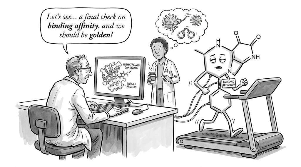
Schrodinger's Desmond molecular dynamics engine is used routinely in pharmaceutical drug design to predict how tightly a candidate molecule binds to its protein target. In the development of nirmatrelvir (Paxlovid's active ingredient against SARS-CoV-2), MD simulations of the drug bound to the 3CL protease active site provided binding free energy estimates that guided medicinal chemists toward modifications improving potency. These simulations ran for hundreds of nanoseconds per compound, generating the kind of trajectory data that the MDAnalysis pipeline in this section is built to process.
The Algorithm That Almost Was Not Published
Daniel Gillespie developed the Stochastic Simulation Algorithm while working at the Naval Weapons Center in China Lake, California, on problems in atmospheric chemistry, not biology. His 1977 paper was initially met with skepticism from chemists who saw no reason to abandon deterministic rate equations. It languished in relative obscurity for over two decades until the rise of systems biology in the early 2000s, when biologists studying gene regulatory networks in single cells realized that the molecule counts were so low (sometimes fewer than 10 copies of a transcription factor) that deterministic models were qualitatively wrong. The paper's citation count exploded from a few dozen to over 10,000. Gillespie himself remarked that he never expected his algorithm to find its main audience in a field he knew nothing about when he wrote it.
Lab: Stochastic Extinction in Predator-Prey Systems
Goal: Measure how the probability of species extinction depends on initial population size in a stochastic Lotka-Volterra system, and compare with the deterministic ODE prediction (which never predicts extinction).
Tools: Python with NumPy and SciPy (scipy.integrate.solve_ivp). Use the gillespie_ssa function from this section.
Procedure: For each initial population size \(N_0 \in \{10, 25, 50, 100, 200, 500\}\), set prey \(= N_0\) and predators \(= N_0 / 2\). Run 100 Gillespie replicate trajectories to \(t_{\max} = 200\) using the Lotka-Volterra reactions defined in this section. Record whether either species goes extinct (count reaches zero) in each run. Plot the extinction probability as a function of \(N_0\).
What to vary: Try different rate constant ratios (increase \(c_2\) relative to \(c_1\) and \(c_3\)) and observe how the extinction curve shifts.
What to observe: You should find that extinction probability approaches 1.0 for small \(N_0\) and drops sharply as \(N_0\) increases, with a characteristic threshold population below which stochastic extinction is almost certain. The deterministic ODE (which you can solve with solve_ivp for comparison) predicts perfectly stable cycles regardless of \(N_0\). This divergence between stochastic and deterministic models is the central lesson: for small populations, the mean-field approximation is not just imprecise but qualitatively misleading.
What's Next
Section 43.3: Simulator Calibration tackles the inverse problem: given observed data, what parameter values make your simulator reproduce reality? When the simulator has no tractable likelihood function (as is the case for all the simulators in this section), Approximate Bayesian Computation provides a principled, likelihood-free solution.