"You want me to find the parameters that make my simulation match your data? Easy. You want a posterior distribution over those parameters? That is what keeps me up at night."
A Likelihood Function That Refused to Be Evaluated
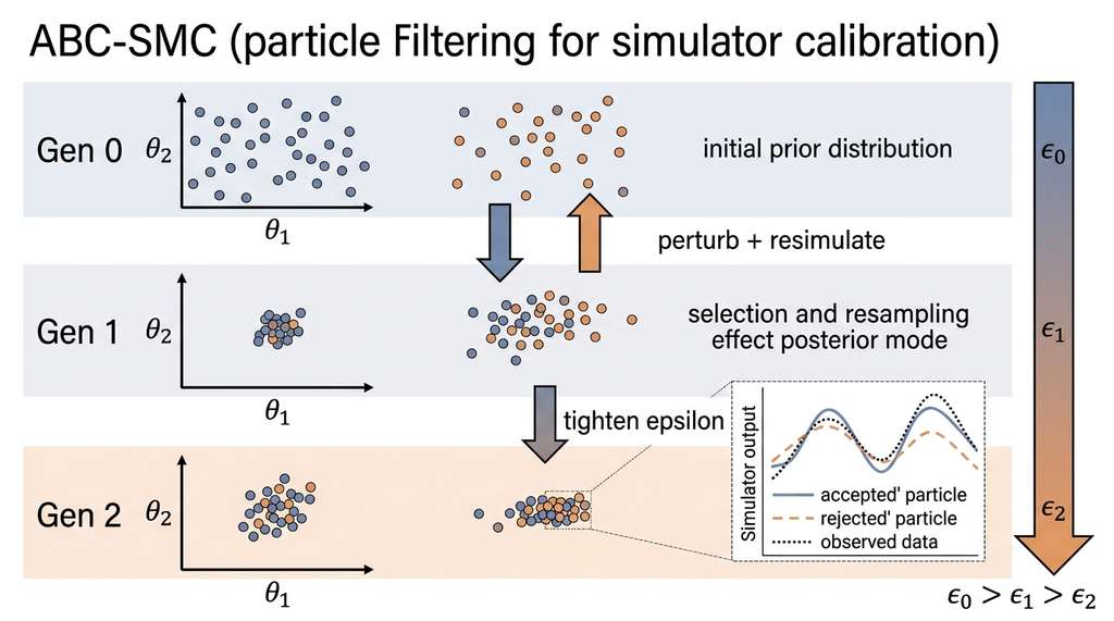
Every simulator has parameters. The Gillespie algorithm has rate constants. Molecular dynamics has force field parameters. Agent-based models have behavioral thresholds. Calibration is the process of finding parameter values that make the simulator's output match observed data. For simple models, you can write down a likelihood function and apply standard Bayesian inference. For the simulators in this chapter, you cannot: the likelihood function is either intractable (no closed-form expression) or computationally prohibitive. Approximate Bayesian Computation (ABC) solves this problem by replacing likelihood evaluation with simulation: if the simulator's output is "close enough" to the data, accept the parameters. ABC-SMC (ABC combined with Sequential Monte Carlo) refines this idea with sequential particle filtering, converging efficiently to the posterior distribution. Figure 43.3.1 below illustrates how ABC-SMC progressively narrows the parameter search across generations.
1. The Calibration Problem
Your climate model has fourteen free parameters, and none of the combinations you have tried reproduce last century's temperature record. Your epidemiological simulator matches case counts only if you hand-tune three rate constants to four decimal places. In both cases, the real question is the same: which parameter values would make the simulator match observed reality? And how much should you trust the answer?
Calibration is the inverse of simulation. Simulation maps parameters to data: given \(\theta\), run the simulator and produce synthetic observations \(\mathbf{y}_{\text{sim}}\). Calibration maps data to parameters: given real observations \(\mathbf{y}_{\text{obs}}\), find the \(\theta\) that could have produced them.
What. Simulator calibration infers the posterior distribution \(p(\theta \mid \mathbf{y}_{\text{obs}})\) over parameters \(\theta\) given observed data \(\mathbf{y}_{\text{obs}}\), using Bayes' theorem:
$$p(\theta \mid \mathbf{y}_{\text{obs}}) = \frac{p(\mathbf{y}_{\text{obs}} \mid \theta) \, p(\theta)}{p(\mathbf{y}_{\text{obs}})}$$Why. Point estimates of parameters (e.g., from least-squares fitting) tell you the single best-fit value but hide the uncertainty. A posterior distribution tells you which parameter regions are consistent with the data and which are ruled out. This matters for prediction: if the posterior is wide, predictions will be uncertain; if it is narrow, predictions are reliable. It also matters for model comparison, a topic we touched on in Chapter 32.
How. Standard Bayesian inference evaluates the likelihood \(p(\mathbf{y}_{\text{obs}} \mid \theta)\), the probability of observing the data given the parameters. For a Gillespie simulation, computing this likelihood requires summing over all possible reaction sequences that produce the observed trajectory, a combinatorial explosion. For molecular dynamics, it requires integrating over all atomic trajectories consistent with the observed macroscopic properties. In both cases, the likelihood is intractable.
When. Use likelihood-free methods whenever you have a simulator that can generate synthetic data but cannot evaluate the probability of specific observations. This includes virtually all stochastic simulators, agent-based models, and molecular dynamics engines. In short: if you can run the simulator forward but cannot write down how probable the data is, simulate your way to the posterior.
The inability to evaluate a likelihood function was once a dead end for Bayesian inference. ABC changed this by observing that you do not need the likelihood if you can simulate from the model. Instead of asking "How probable is the data given these parameters?" you ask "Can the simulator produce data that looks like the observations?" This shift from evaluation to simulation opened Bayesian inference to an enormous class of models that were previously inaccessible: population genetics, epidemiology, ecology, systems biology, and cosmology all adopted ABC within a decade of its introduction.
2. ABC Rejection Sampling
Standard likelihood evaluation fails for complex simulators, so the practical question becomes: what replaces it?
When a climate model's parameters are even slightly off, it can project sea-level rise a full meter too high or too low, turning a policy decision into a coin flip. Getting calibration wrong does not just produce a bad fit; it produces confident predictions that mislead.
The simplest ABC algorithm is rejection sampling. The idea is to sample parameters from the prior, run the simulator, and keep only those parameter values whose simulated output is "close enough" to the observed data. "Close enough" is formalized through a distance function and a tolerance threshold.
Mental Model
Think of ABC rejection sampling as a detective reconstructing a recipe by tasting the final dish. The detective cannot reverse-engineer the cooking process step by step (the likelihood is intractable), so instead she tries hundreds of candidate recipes, cooks each one, and tastes the result. If a candidate dish tastes "close enough" to the original, the recipe is kept as plausible; otherwise it is discarded. Tightening the tolerance is like demanding a closer flavor match: fewer recipes survive, but the survivors are more faithful. The key mechanism is the same: replace an impossible backward calculation with many forward trials followed by a comparison.
The algorithm:
- Draw \(\theta^* \sim p(\theta)\) from the prior distribution.
- Simulate: \(\mathbf{y}^* \sim p(\mathbf{y} \mid \theta^*)\) by running the simulator with parameters \(\theta^*\).
- Compute summary statistics: \(s^* = S(\mathbf{y}^*)\) and \(s_{\text{obs}} = S(\mathbf{y}_{\text{obs}})\), where \(S(\cdot)\) is a deterministic function that compresses high-dimensional simulator output into a fixed-length numeric vector.
- Compute the distance: \(d = \rho(s^*, s_{\text{obs}})\).
- If \(d \leq \epsilon\) (the tolerance), accept \(\theta^*\); otherwise reject.
- Repeat until you have enough accepted samples.
The accepted samples approximate the ABC posterior \(p_\epsilon(\theta \mid s_{\text{obs}})\), which converges to the true posterior as \(\epsilon \to 0\) (assuming the summary statistics are sufficient, where a sufficient statistic is one that captures all information in the data relevant to the parameters). In practice, \(\epsilon\) is always positive, introducing an approximation whose quality depends on the choice of summary statistics and distance function.
import numpy as np
from scipy.spatial.distance import euclidean


def abc_rejection(
    simulator_fn,
    summary_fn,
    observed_summaries,
    prior_sampler,
    epsilon,
    n_accepted=1000,
    max_iterations=1_000_000,
    seed=42,
):
    """ABC rejection sampling for likelihood-free inference.

    Args:
        simulator_fn: callable(params, seed) -> simulated data
        summary_fn: callable(data) -> summary statistics vector
        observed_summaries: summary statistics of the observed data
        prior_sampler: callable(rng) -> parameter vector from the prior
        epsilon: acceptance threshold
        n_accepted: target number of accepted samples
        max_iterations: safety limit on total simulations
        seed: random seed

    Returns:
        accepted_params: array of shape (n_accepted, n_params)
        acceptance_rate: fraction of simulations accepted
    """
    rng = np.random.default_rng(seed)
    accepted = []
    n_total = 0

    while len(accepted) < n_accepted and n_total < max_iterations:
        # Step 1: Sample from prior
        theta = prior_sampler(rng)

        # Step 2: Simulate
        sim_seed = rng.integers(0, 2**31)
        sim_data = simulator_fn(theta, seed=sim_seed)

        # Step 3: Compute summary statistics
        sim_summaries = summary_fn(sim_data)

        # Step 4: Accept/reject
        distance = euclidean(sim_summaries, observed_summaries)
        if distance <= epsilon:
            accepted.append(theta)

        n_total += 1

    accepted_params = np.array(accepted)
    acceptance_rate = len(accepted) / n_total

    print(f"ABC rejection: {len(accepted)}/{n_total} accepted "
          f"(rate={acceptance_rate:.4f})")

return accepted_params, acceptance_rate2.1 Choosing Summary Statistics
The summary statistics \(S(\mathbf{y})\) are the most consequential design choice in ABC. Ideally, they would be sufficient statistics: functions that capture all the information in the data relevant to the parameters. In practice, sufficient statistics are rarely known for complex simulators, so you must choose informative but computable summaries.
Summary statistics are deterministic functions that compress a simulator's raw output into a fixed-length numeric vector. That output may be a high-dimensional time series, a spatial field, or a variable-length event log. Summary statistics matter because ABC compares simulated and observed data exclusively through these compressed representations. Any information lost during compression is invisible to the inference and can never be recovered, no matter how many simulations you run. The mechanism is straightforward: apply the same function \(S(\cdot)\) to both the observed data and each simulated dataset, then measure the distance between the two resulting vectors. Use hand-crafted summary statistics when domain knowledge identifies which data features carry parameter information. Switch to learned summaries (Section 6) when the parameter-to-data mapping is too complex for manual feature engineering, or when calibration checks reveal that hand-crafted summaries miss important structure.
For a stochastic biochemical system, good summary statistics typically include:
- Moments: mean, variance, and covariance of species counts at specific time points.
- Temporal features: autocorrelation at lag 1, period of oscillations (if present), time to steady state.
- Distributional features: quantiles (10th, 50th, 90th percentiles) of species counts at equilibrium.
- Event statistics: frequency of extinction events, time of first passage to a threshold.
def biochemical_summary_statistics(trajectory, t_eval=None):
    """Compute summary statistics for a stochastic biochemical trajectory.

    Args:
        trajectory: dict with 'times' and 'states' arrays
        t_eval: time points at which to evaluate (default: use all)

    Returns:
        summary: 1D array of summary statistics
    """
    times = trajectory["times"]
    states = trajectory["states"]
    n_species = states.shape[1]

    summaries = []

    for s in range(n_species):
        series = states[:, s]

        # Moments
        summaries.append(np.mean(series))
        summaries.append(np.std(series))

        # Quantiles
        summaries.extend(np.percentile(series, [10, 50, 90]).tolist())

        # Temporal: autocorrelation at lag 1
        if len(series) > 1:
            centered = series - np.mean(series)
            var = np.var(series)
            if var > 0:
                ac1 = np.correlate(centered[:-1], centered[1:])[0]
                ac1 /= (len(centered) - 1) * var
            else:
                ac1 = 0.0
            summaries.append(ac1)
        else:
            summaries.append(0.0)

    # Cross-species correlation (if multiple species)
    if n_species >= 2:
        corr = np.corrcoef(states[:, 0], states[:, 1])[0, 1]
        summaries.append(corr if np.isfinite(corr) else 0.0)

return np.array(summaries)If your summary statistics discard information about the parameters, the ABC posterior will be wider than the true posterior (loss of precision) or, worse, centered on the wrong value (bias). A classic failure mode is using only the mean of a distribution when the variance also depends on the parameters. Always include at least one summary statistic per parameter you are trying to infer, and validate your choice by running ABC on synthetic data with known parameters (a "calibration check") before applying it to real data.
Common Misconception
Readers often assume that making the tolerance \(\epsilon\) as small as possible always produces a better posterior. In reality, a very tight \(\epsilon\) combined with insufficient summary statistics can produce a posterior that is both narrow and wrong: it concentrates confidently around incorrect parameter values because the summary statistics cannot distinguish the true parameters from nearby impostors. The correct practice is to validate summary statistic quality first (via calibration checks on synthetic data with known parameters) and only then tighten \(\epsilon\); a well-chosen set of summaries at moderate tolerance outperforms a poor set of summaries at any tolerance.
Step-Through: ABC Rejection on a Toy Model
Trace through ABC rejection sampling for a simulator that produces a single number drawn from \(\mathcal{N}(\theta, 1)\), with observed data \(y_{\text{obs}} = 3.0\), summary statistic = sample mean (of 10 draws), tolerance \(\epsilon = 1.5\), and a uniform prior \(\theta \sim U(0, 6)\).
Iteration 1: Draw \(\theta^* = 4.8\). Simulate 10 draws from \(\mathcal{N}(4.8, 1)\), get mean \(s^* = 5.12\). Distance \(|5.12 - 3.0| = 2.12 > 1.5\). Reject.
Iteration 2: Draw \(\theta^* = 2.3\). Simulate, get mean \(s^* = 2.47\). Distance \(|2.47 - 3.0| = 0.53 \leq 1.5\). Accept.
Iteration 3: Draw \(\theta^* = 0.6\). Simulate, get mean \(s^* = 0.71\). Distance \(|0.71 - 3.0| = 2.29 > 1.5\). Reject.
Iteration 4: Draw \(\theta^* = 3.5\). Simulate, get mean \(s^* = 3.22\). Distance \(|3.22 - 3.0| = 0.22 \leq 1.5\). Accept.
After many iterations, the accepted \(\theta\) values cluster around 3.0, forming the approximate posterior. Tightening \(\epsilon\) to 0.5 would reject iteration 2 as well (\(0.53 > 0.5\)), producing a sharper posterior at the cost of a lower acceptance rate.
Exercise 43.3.1
A researcher runs ABC rejection sampling on a two-parameter model with tolerance \(\epsilon = 1.0\) and observes an acceptance rate of 0.2%. She then switches from Euclidean distance to Mahalanobis distance, where the Mahalanobis distance normalizes each summary statistic dimension by its variance so that all dimensions contribute equally, and the acceptance rate jumps to 1.8% at the same nominal \(\epsilon\). Explain why the distance metric change affects the acceptance rate, and state whether the resulting posterior from the Mahalanobis variant is necessarily better. Under what condition could the higher acceptance rate actually indicate a worse posterior approximation?
Hint
Consider what happens when summary statistics have very different variances. Euclidean distance is dominated by the statistic with the largest absolute scale, effectively ignoring the others. Mahalanobis distance normalizes each dimension. Think about whether a higher acceptance rate always means you are sampling from a distribution closer to the true posterior, or whether it could mean you are being less selective along dimensions that carry parameter information.
3. ABC-SMC: Sequential Monte Carlo for Efficient Calibration
ABC rejection sampling has a fatal scalability problem: as you tighten \(\epsilon\) to improve accuracy, the acceptance rate drops exponentially. With three parameters and a moderately tight tolerance, acceptance rates below 0.01% are not unusual, meaning you need millions of simulations to collect a thousand posterior samples.
ABC-SMC (Sequential Monte Carlo) solves this by replacing the single, harsh rejection step with a sequence of increasingly strict filtering rounds. Each round starts from the accepted particles of the previous round (not the prior), so the proposal distribution is always concentrated near the posterior. The algorithm uses importance weights (scalar corrections assigned to each particle so that the resampled population still represents the correct target distribution, compensating for the fact that particles were proposed from the previous generation rather than from the prior), along with a perturbation kernel (a probability distribution, typically Gaussian, used to jitter each particle to a nearby location in parameter space) to maintain proper sampling. Figure 43.3.1 shows this sequential narrowing process.
The algorithm:
- Generation 0: Run ABC rejection with a generous tolerance \(\epsilon_0\). The accepted particles form the initial population.
- Generation \(t\): For each particle in the new population:
- Sample a particle \(\theta^{**}\) from the previous generation's population (with weights).
- Perturb: \(\theta^* = \theta^{**} + K\), where \(K\) is drawn from a perturbation kernel (typically Gaussian).
- If \(\theta^*\) has zero prior probability, return to (a).
- Simulate and compute summary statistics.
- If \(\rho(s^*, s_{\text{obs}}) \leq \epsilon_t\), accept \(\theta^*\); otherwise return to (a).
- Assign weight: \(w^* = p(\theta^*) \big/ \sum_{j} w_j^{(t-1)} K(\theta^* \mid \theta_j^{(t-1)})\). Intuitively, this ratio is large when the prior favors \(\theta^*\) but the previous generation's particles do not, upweighting regions the perturbation kernel undersampled.
- Decrease \(\epsilon_t\) and repeat until convergence or budget exhaustion.
from scipy.stats import gaussian_kde


def abc_smc(
    simulator_fn,
    summary_fn,
    observed_summaries,
    prior_sampler,
    prior_pdf,
    epsilons,
    n_particles=500,
    seed=42,
):
    """ABC-SMC for efficient likelihood-free posterior inference.

    Args:
        simulator_fn: callable(params, seed) -> simulated data
        summary_fn: callable(data) -> summary statistics vector
        observed_summaries: summary statistics of the observed data
        prior_sampler: callable(rng) -> parameter vector from the prior
        prior_pdf: callable(params) -> prior density at params
        epsilons: decreasing sequence of tolerance thresholds
        n_particles: number of particles per generation
        seed: random seed

    Returns:
        particles: final population, shape (n_particles, n_params)
        weights: normalized importance weights
        all_populations: list of populations from each generation
    """
    rng = np.random.default_rng(seed)
    all_populations = []

    # Generation 0: ABC rejection with epsilon[0]
    particles = []
    while len(particles) < n_particles:
        theta = prior_sampler(rng)
        sim_data = simulator_fn(theta, seed=rng.integers(0, 2**31))
        sim_summary = summary_fn(sim_data)
        if euclidean(sim_summary, observed_summaries) <= epsilons[0]:
            particles.append(theta)

    particles = np.array(particles)
    weights = np.ones(n_particles) / n_particles
    all_populations.append(particles.copy())
    print(f"Gen 0: eps={epsilons[0]:.4f}, {n_particles} particles accepted")

    # Subsequent generations
    for gen, eps in enumerate(epsilons[1:], start=1):
        # Compute perturbation kernel bandwidth from previous population
        n_params = particles.shape[1]
        cov = 2.0 * np.cov(particles.T, aweights=weights)

        new_particles = []
        new_weights_raw = []

        while len(new_particles) < n_particles:
            # Sample a particle from previous generation
            idx = rng.choice(n_particles, p=weights)
            theta_star = particles[idx]

            # Perturb
            theta_proposed = rng.multivariate_normal(theta_star, cov)

            # Check prior support
            if prior_pdf(theta_proposed) == 0:
                continue

            # Simulate
            sim_data = simulator_fn(
                theta_proposed, seed=rng.integers(0, 2**31)
            )
            sim_summary = summary_fn(sim_data)

            if euclidean(sim_summary, observed_summaries) <= eps:
                new_particles.append(theta_proposed)

                # Importance weight
                kernel_sum = 0.0
                for j in range(n_particles):
                    diff = theta_proposed - particles[j]
                    kernel_sum += weights[j] * np.exp(
                        -0.5 * diff @ np.linalg.solve(cov, diff)
                    )
                w = prior_pdf(theta_proposed) / kernel_sum
                new_weights_raw.append(w)

        particles = np.array(new_particles)
        weights = np.array(new_weights_raw)
        weights /= weights.sum()
        all_populations.append(particles.copy())
        print(f"Gen {gen}: eps={eps:.4f}, {n_particles} particles accepted")

    return particles, weights, all_populations
ABC-SMC applies the same particle filtering logic that sequential Monte Carlo uses for state estimation in hidden Markov models. Each "particle" is a candidate parameter vector. The "observation" is the real data's summary statistics. The "transition" is the perturbation kernel. The "likelihood" is replaced by the accept/reject decision. If you have studied particle filters in signal processing or robotics, ABC-SMC is the same algorithm applied to the parameter space of a simulator rather than the state space of a dynamical system. This connection to Chapter 32's Bayesian methods is not superficial; it is the same mathematical framework.
4. pyABC: Production-Grade ABC-SMC
The implementation above illustrates the algorithm, but production calibration requires features that a textbook implementation lacks: adaptive epsilon schedules, distributed computing, early termination, model selection, and diagnostics. The pyABC library provides all of these.
import pyabc
from pyabc import (
    ABCSMC, RV, Distribution,
    MedianEpsilon, LocalTransition,
)
import tempfile
import os


def calibrate_with_pyabc(
    simulator_fn,
    summary_fn,
    observed_summaries,
    param_priors,
    n_populations=10,
    min_epsilon=0.1,
    population_size=200,
):
    """Calibrate a simulator using pyABC's ABC-SMC implementation.

    Args:
        simulator_fn: callable(params_dict) -> simulated data
        summary_fn: callable(data) -> dict of summary statistics
        observed_summaries: dict of observed summary statistics
        param_priors: dict mapping param name to pyabc.RV distribution
        n_populations: maximum number of SMC generations
        min_epsilon: stop when epsilon falls below this value
        population_size: particles per generation

    Returns:
        history: pyABC History object with all generations
    """
    # Define the prior
    prior = Distribution(**param_priors)

    # Define the model (simulator + summary statistics)
    def model(params):
        sim_data = simulator_fn(params)
        return summary_fn(sim_data)

    # Distance function: weighted Euclidean
    distance = pyabc.AdaptivePNormDistance(p=2)

    # Epsilon schedule: adaptive median
    epsilon = MedianEpsilon(initial_epsilon=50.0)

    # Perturbation kernel: local (adapts to particle spread)
    transition = LocalTransition(k_fraction=0.25)

    # Create the ABC-SMC object
    abc = ABCSMC(
        models=model,
        parameter_priors=prior,
        distance_function=distance,
        population_size=population_size,
        transitions=transition,
        eps=epsilon,
    )

    # Database for storing results
    db_path = os.path.join(tempfile.gettempdir(), "abc_calibration.db")
    abc.new(f"sqlite:///{db_path}", observed_summaries)

    # Run the inference
    history = abc.run(
        minimum_epsilon=min_epsilon,
        max_nr_populations=n_populations,
    )

    print(f"Calibration complete: {history.n_populations} generations")
    print(f"Final epsilon: {history.get_all_populations()['epsilon'].min():.4f}")

    return history


# Example usage with the Lotka-Volterra system
param_priors = {
    "prey_birth": RV("uniform", 0.1, 1.5),
    "predation": RV("uniform", 0.001, 0.02),
    "predator_death": RV("uniform", 0.05, 0.8),
}

# In practice, you would pass your actual simulator and observed data:
# history = calibrate_with_pyabc(
#     simulator_fn=lotka_volterra_simulator,
#     summary_fn=compute_summaries,
#     observed_summaries={"mean_prey": 85.0, "mean_pred": 42.0, ...},
#     param_priors=param_priors,
# )The manual ABC-SMC implementation above requires roughly 80 lines for the core algorithm plus additional code for epsilon scheduling, kernel adaptation, convergence diagnostics, serialization, and parallelism. pyABC provides all of this in about 20 lines of setup code. It also supports model selection (comparing multiple competing simulators), look-ahead scheduling for distributed computing, and integration with Redis for multi-machine parallelism. The library handles the sampling infrastructure; you provide the simulator, the summary statistics, and the prior.
5. Diagnostics: Is the Calibration Trustworthy?
A calibration is only as good as its validation. Three diagnostic checks should be routine.
5.1 Prior Predictive Check
Before running ABC, verify that the prior is broad enough to include the data-generating parameters. Simulate from the prior and check that the observed summary statistics fall within the range of simulated summaries.
def prior_predictive_check(
    simulator_fn, summary_fn, prior_sampler, observed_summaries,
    n_samples=1000, seed=42,
):
    """Check that the prior covers the observed data.

    Returns the fraction of summary statistics for which the
    observed value falls within the prior predictive range.
    """
    rng = np.random.default_rng(seed)
    sim_summaries = []

    for _ in range(n_samples):
        theta = prior_sampler(rng)
        sim_data = simulator_fn(theta, seed=rng.integers(0, 2**31))
        sim_summaries.append(summary_fn(sim_data))

    sim_summaries = np.array(sim_summaries)
    n_stats = len(observed_summaries)
    covered = 0

    for j in range(n_stats):
        lo, hi = np.percentile(sim_summaries[:, j], [1, 99])
        if lo <= observed_summaries[j] <= hi:
            covered += 1

    coverage = covered / n_stats
    print(f"Prior predictive coverage: {covered}/{n_stats} "
          f"statistics covered ({coverage:.0%})")
return coverage5.2 Posterior Predictive Check
After calibration, simulate from the posterior and compare the simulated summary statistics to the observed ones. If they match well, the calibration is consistent. If they do not, either the summary statistics are insufficient or the model is misspecified.
def posterior_predictive_check(
    simulator_fn, summary_fn, posterior_samples, observed_summaries,
    n_simulations_per_sample=5, seed=42,
):
    """Validate calibration by simulating from the posterior.

    Returns the distribution of distances between posterior-predictive
    summaries and the observed summaries.
    """
    rng = np.random.default_rng(seed)
    distances = []

    for theta in posterior_samples:
        for _ in range(n_simulations_per_sample):
            sim_data = simulator_fn(theta, seed=rng.integers(0, 2**31))
            sim_summary = summary_fn(sim_data)
            d = euclidean(sim_summary, observed_summaries)
            distances.append(d)

    distances = np.array(distances)
    print(f"Posterior predictive distances: "
          f"median={np.median(distances):.4f}, "
          f"p95={np.percentile(distances, 95):.4f}")
return distances5.3 Calibration on Synthetic Data
The gold-standard diagnostic is to run the entire calibration pipeline on synthetic data generated with known parameters. If the posterior concentrates around the true values, the pipeline is working. If it does not, debug before applying to real data.
def calibration_check(
    simulator_fn, summary_fn, prior_sampler, prior_pdf,
    true_params, epsilons, n_particles=300, seed=42,
):
    """Run ABC-SMC on synthetic data with known true parameters.

    The posterior should concentrate around true_params if the
    summary statistics are informative and the model is correct.
    """
    rng = np.random.default_rng(seed)

    # Generate "observed" data from true parameters
    observed_data = simulator_fn(true_params, seed=rng.integers(0, 2**31))
    observed_summaries = summary_fn(observed_data)

    # Run ABC-SMC
    particles, weights, _ = abc_smc(
        simulator_fn=simulator_fn,
        summary_fn=summary_fn,
        observed_summaries=observed_summaries,
        prior_sampler=prior_sampler,
        prior_pdf=prior_pdf,
        epsilons=epsilons,
        n_particles=n_particles,
        seed=seed + 1,
    )

    # Check: is the true value within the 95% credible region?
    for j in range(len(true_params)):
        weighted_mean = np.average(particles[:, j], weights=weights)
        lo = np.percentile(particles[:, j], 2.5)
        hi = np.percentile(particles[:, j], 97.5)
        covered = lo <= true_params[j] <= hi
        print(
            f"Param {j}: true={true_params[j]:.4f}, "
            f"posterior mean={weighted_mean:.4f}, "
            f"95% CI=[{lo:.4f}, {hi:.4f}], "
            f"covered={covered}"
        )

return particles, weightsDuring the early weeks of a novel pathogen outbreak, epidemiologists must estimate the basic reproduction number \(R_0\) (the average number of secondary infections caused by a single infected individual in a fully susceptible population) and the serial interval from sparse, noisy case data. The SEIR (Susceptible-Exposed-Infected-Recovered) model is a standard simulator, but its likelihood is intractable because the infection times are unobserved. ABC-SMC calibration with summary statistics (daily case counts, growth rate, generation interval distribution) provides posterior distributions over \(R_0\) and other parameters within hours. The UK's Real-Time Assessment of Community Transmission (REACT) study used ABC-based calibration to provide weekly estimates of transmission rates during the COVID-19 pandemic, contributing to policy discussions on school closures and lockdown timing.
Real-World Application: Cosmological Parameter Estimation
Cosmological parameter estimation has adopted ABC-based methods to calibrate simulators against cosmic microwave background (CMB) power spectra, inferring posterior distributions over parameters such as the Hubble constant \(H_0\), baryon density, and dark energy equation of state. While the Planck Collaboration primarily used Markov chain Monte Carlo via CosmoMC, independent groups (notably Akeret et al., 2015; Ishida et al., 2015) demonstrated that ABC-SMC can recover comparable posteriors when the full CMB likelihood, which involves a computationally expensive Boltzmann solver (CLASS or CAMB), is replaced by angular power spectrum summary statistics.
The Algorithm That Was Invented Twice
ABC was independently proposed by geneticists (Tavaré et al., 1997) and ecologists (Pritchard et al., 1999) within two years, neither group aware of the other. Both faced the same problem: population genetics simulators that could generate synthetic genealogies but could not evaluate the probability of observed gene frequencies. The geneticists called their method "simulation-based inference"; the ecologists called it "approximate Bayesian computation." The ecology name stuck, but the genetics paper came first. Even more remarkably, a nearly identical idea appeared in a 1984 paper by Peter Diggle and Richard Gratton on indirect inference for spatial point processes, but lay dormant for over a decade because the computational power to run thousands of simulations did not exist yet.
6. Advanced Topics: Adaptive Summary Statistics
The diagnostics above repeatedly highlight one theme: calibration quality depends on the summary statistics, and a poor choice cannot be rescued by tighter tolerances or more simulations.
Choosing summary statistics by hand requires domain expertise and risks missing informative features. Recent work automates this step using neural networks trained to extract maximally informative summaries from simulated data.
The idea is to train a neural network \(f_\phi\) that maps raw simulation output to a low-dimensional embedding, where the embedding is trained to be maximally informative about the parameters \(\theta\). Two approaches dominate:
Two Dominant Approaches
Semi-automatic ABC (Fearnhead and Prangle, 2012): Train a regression model to predict \(\theta\) from the raw data. The predicted values \(\hat{\theta}\) serve as summary statistics, which, under regularity conditions on the regression model, are approximately sufficient.
Neural posterior estimation (Papamakarios and Murray, 2016): Train a conditional density network (a neural network that outputs not a single prediction but an entire probability distribution over \(\theta\), conditioned on the observed data) to estimate \(p(\theta \mid \mathbf{y})\) directly, bypassing ABC entirely. This approach, sometimes called "simulation-based inference" (SBI), is covered in detail in packages like sbi (Tejero-Cantero et al., 2020) and represents the frontier of likelihood-free inference.
Checkpoint
So far: hand-crafted summary statistics can be replaced by learned ones, either through a regression network whose bottleneck layer serves as approximately sufficient summaries (semi-automatic ABC) or through a conditional density network that estimates the full posterior directly, bypassing the ABC accept/reject loop entirely (neural posterior estimation).
Research Frontier
Flow matching for simulation-based inference (FMPE, Wildberger et al., 2024) replaces the normalizing-flow density estimators used in earlier neural posterior estimation with continuous normalizing flows trained via flow matching objectives. The method, published at ICML 2024 as "Flow Matching for Scalable Simulation-Based Inference," achieves state-of-the-art posterior approximation quality on standard SBI benchmarks while training significantly faster than comparable normalizing-flow approaches. It also scales more gracefully to high-dimensional parameter spaces (tested up to 100 dimensions) where traditional ABC-SMC becomes computationally infeasible. The sbi Python package (v0.22+) includes FMPE as a built-in method, making it accessible without custom implementation. As of 2025, sbi has reached v0.23+ and consolidated several neural posterior estimation backends, including FMPE, under a unified API; check the current documentation for the latest method names and defaults.
def train_summary_network(
    simulator_fn, prior_sampler, n_train=10_000, n_summary_dims=5,
    seed=42,
):
    """Train a neural network to learn informative summary statistics.

    Uses a simple regression approach: the network learns to predict
    parameters from raw simulation output. The network's penultimate
    layer provides learned summary statistics.
    """
    import torch
    import torch.nn as nn

    rng = np.random.default_rng(seed)

    # Generate training data: (simulation output, true parameters)
    X_list, y_list = [], []
    for _ in range(n_train):
        theta = prior_sampler(rng)
        sim_data = simulator_fn(theta, seed=rng.integers(0, 2**31))
        # Flatten simulation output to a fixed-size vector
        flat = np.concatenate([
            np.mean(sim_data["states"], axis=0),
            np.std(sim_data["states"], axis=0),
            np.percentile(sim_data["states"], [25, 75], axis=0).flatten(),
        ])
        X_list.append(flat)
        y_list.append(theta)

    X = torch.tensor(np.array(X_list), dtype=torch.float32)
    y = torch.tensor(np.array(y_list), dtype=torch.float32)

    # Simple regression network
    input_dim = X.shape[1]
    param_dim = y.shape[1]

    model = nn.Sequential(
        nn.Linear(input_dim, 64),
        nn.ReLU(),
        nn.Linear(64, n_summary_dims),  # learned summaries
        nn.ReLU(),
        nn.Linear(n_summary_dims, param_dim),
    )

    optimizer = torch.optim.Adam(model.parameters(), lr=1e-3)
    loss_fn = nn.MSELoss()

    # Training loop
    for epoch in range(200):
        optimizer.zero_grad()
        pred = model(X)
        loss = loss_fn(pred, y)
        loss.backward()
        optimizer.step()
        if (epoch + 1) % 50 == 0:
            print(f"Epoch {epoch+1}: loss={loss.item():.4f}")

    # Extract the summary network (everything up to the bottleneck)
    summary_net = nn.Sequential(*list(model.children())[:3])
return summary_net, modelTry It: ABC Calibration of a Gaussian Mixture
Build a complete ABC rejection sampler for a two-component Gaussian mixture model using only NumPy and SciPy. This exercise isolates the calibration logic from simulator complexity so you can focus on the ABC workflow itself.
- Define a simulator. Write a function that takes parameters \(\theta = (\mu_1, \mu_2, w)\) (two means and a mixing weight) and generates \(n=200\) samples from the mixture \(w \cdot \mathcal{N}(\mu_1, 1) + (1 - w) \cdot \mathcal{N}(\mu_2, 1)\).
- Choose summary statistics. Implement a summary function that computes five quantities from a sample: the sample mean, sample variance, skewness (
scipy.stats.skew), the 25th percentile, and the 75th percentile. - Generate synthetic "observed" data. Fix true parameters (e.g., \(\mu_1 = -2\), \(\mu_2 = 3\), \(w = 0.4\)), run the simulator once, and compute observed summaries.
- Run ABC rejection. Sample 100,000 candidate parameter vectors from uniform priors (\(\mu_i \in [-5, 5]\), \(w \in [0, 1]\)), simulate each, and accept those with Euclidean summary distance below a threshold \(\epsilon\). Start with \(\epsilon = 2.0\) and tighten to \(\epsilon = 0.5\). Plot histograms of accepted \(\mu_1\), \(\mu_2\), and \(w\) values using
matplotlib. - Validate. Check whether the true parameter values fall within the central 95% of each accepted-parameter histogram. If not, add more summary statistics (e.g., bimodality coefficient or kernel density mode count) and repeat.
7. Summary
Simulator calibration inverts a forward model: given observed data, recover the posterior over parameters. When the likelihood is intractable, ABC offers an alternative: simulate, summarize, compare. ABC-SMC refines this through sequential particle filtering with decreasing tolerances, as illustrated in Figure 43.3.1. Calibration quality hinges on summary statistics, whether hand-crafted or learned. Diagnostic checks (prior predictive, posterior predictive, synthetic-data calibration) are the only way to verify trustworthiness. The next section assembles these components into a complete calibrated simulator pipeline.
Lab: ABC Calibration of a Lotka-Volterra Predator-Prey Model
Goal: Recover known parameters of a stochastic Lotka-Volterra system using ABC rejection sampling, then upgrade to ABC-SMC and compare convergence speed and posterior quality.
Tools needed: Python 3.9+, NumPy, SciPy, matplotlib, and (optionally) pyABC (pip install pyabc).
Setup (5 min): Implement a discrete-time stochastic Lotka-Volterra simulator with three parameters: prey birth rate \(\alpha = 0.5\), predation rate \(\beta = 0.01\), and predator death rate \(\gamma = 0.3\). Generate a 200-step "observed" trajectory from these true values. Compute five summary statistics: mean prey count, mean predator count, standard deviation of each, and cross-correlation.
Phase 1, ABC rejection (10 min): Draw 50,000 parameter samples from uniform priors (\(\alpha \in [0.1, 1.0]\), \(\beta \in [0.001, 0.05]\), \(\gamma \in [0.05, 0.8]\)). Run the simulator for each, accept those within Euclidean distance \(\epsilon = 5.0\) of observed summaries. Plot marginal histograms of accepted parameters and check whether the true values fall inside the 95% range.
Phase 2, ABC-SMC (10 min): Use the abc_smc function from this section (or pyABC) with epsilon schedule \([8, 5, 3, 2, 1]\). Compare the final posterior width to the rejection posterior. Observe how many total simulations each method required to reach the same tolerance.
What to vary: (a) Remove one summary statistic (e.g., cross-correlation) and observe the posterior widening. (b) Add the lag-1 autocorrelation of prey counts and check whether the posterior sharpens. (c) Halve the observed trajectory length to 100 steps and note the effect on posterior uncertainty.
What to observe: The ratio of total simulations between rejection and SMC at matched tolerance, the sensitivity of posterior width to summary statistic choice, and whether all calibration checks pass (true parameters inside the 95% credible interval).
What's Next
Section 43.4: Building a Calibrated Simulator brings together the Gillespie algorithm from Section 43.2, the ABC-SMC calibration from this section, and the Discovery Workbench integration from Section 43.1 into a complete recipe. The workflow calibrates a stochastic model of a gene regulatory network against synthetic experimental data, then use the calibrated model for counterfactual interventions that test mechanistic hypotheses.