Section 33.3: Equivariant Neural Networks

The Big Picture

The energy of a molecule does not change if you rotate it. The forces on its atoms rotate with the molecule. These are not observations to be learned from data; they are mathematical guarantees that follow from the symmetries of physical law. An equivariant neural network encodes these symmetries directly into its architecture, so the network cannot violate them regardless of the training data. The result is dramatic: equivariant models typically achieve the same accuracy as non-equivariant models with 10 to 100 times less training data, and they generalize reliably to molecular configurations never seen during training. This section introduces the mathematical framework of symmetry groups, spherical harmonics, and tensor products, then surveys the architectures (MACE, NequIP, GemNet, EquiformerV2) that dominate molecular property prediction.

1. Symmetry Groups for Physical Systems

Why does a neural network that predicts molecular energy need to see 100,000 rotated copies of the same molecule before it learns that rotation does not change the answer, when a first-year physics student knows it from a single symmetry argument?

Three symmetry groups appear throughout molecular and materials science, each describing a set of transformations under which a system's properties are invariant or transform in a predictable way:

O(3), the orthogonal group in 3D: all rotations and reflections. A 3 x 3 matrix $R$ is in $O(3)$ if $R^T R = I$, meaning $\det(R) = \pm 1$. Physical scalar quantities (energy, charge) are invariant under $O(3)$.
SO(3), the special orthogonal group: rotations only ($\det(R) = +1$). Vector quantities like forces transform under $SO(3)$: if we rotate the molecule by $R$, the force on each atom rotates by the same $R$.
E(3), the Euclidean group: rotations, reflections, and translations. Physical properties do not depend on where you place the molecule in space (translation invariance) or how you orient it (rotation invariance/equivariance).

The distinction between invariance and equivariance is central. A function $f$ is invariant under a group $G$ if $f(g \cdot x) = f(x)$ for all $g \in G$. It is equivariant if $f(g \cdot x) = g \cdot f(x)$; the output transforms in the same way as the input. Energy is invariant (rotating the molecule does not change its energy). Forces are equivariant (rotating the molecule rotates the forces).

Equivariance constrains a function (or neural network layer) so that two paths yield the same result: transform the input then compute, or compute then transform. This matters because the architecture enforces a physical symmetry exactly, rather than requiring the model to learn it statistically. The constraint eliminates an entire class of generalization errors and reduces training data requirements by orders of magnitude. The mechanism is direct: each layer restricts its linear maps and nonlinearities to operations that commute with the group action. Clebsch-Gordan tensor products, for example, interleave features of different rotation orders in a mathematically prescribed way. Use equivariant layers whenever the target quantity has a known transformation law under a symmetry group. Resort to data augmentation or unconstrained architectures only when the relevant symmetry is approximate, unknown, or too complex to encode tractably. In short: if you know the symmetry, encode it; the network should spend its capacity discovering physics, not rediscovering geometry.

Key Insight: Why Equivariance Beats Data Augmentation

A non-equivariant network can approximate equivariant behavior through data augmentation: train on randomly rotated copies of each molecule. But this approach has fundamental limitations. First, it is statistically inefficient: the network must "discover" the rotation symmetry from data, spending capacity on a property that could be guaranteed architecturally. Second, the equivariance is approximate, not exact: the network may produce slightly different energies for two orientations of the same molecule. Third, augmentation does not scale: the rotation group $SO(3)$ is continuous and three-dimensional, so no finite set of augmentations covers it. Built-in equivariance eliminates all three problems. As demonstrated in the representation learning framework of Chapter 26, the right inductive bias is always preferable to brute-force data expansion.

Common Misconception

Misconception: "Equivariant networks can only output quantities that are symmetric (unchanged) under the group." This conflates invariance with equivariance. An equivariant network can predict quantities that change under transformations, as long as they change in the correct, predictable way. For instance, an E(3)-equivariant model predicts force vectors that rotate when the molecule rotates; the forces are not invariant, but the model's prediction transforms consistently with the input, which is exactly what equivariance guarantees.

2. Irreducible Representations and Spherical Harmonics

With the symmetry groups defined, the next question is practical: how do we tell a neural network layer which quantities are scalars, which are vectors, and which are higher-order tensors, so that each transforms correctly under rotation?

To build equivariant layers, we need a mathematical language for describing how quantities transform under rotations. The key concept is the irreducible representation (irrep) of $SO(3)$, where an irreducible representation is the smallest matrix representation of the group that cannot be decomposed into simpler ones . Each irrep is indexed by a non-negative integer $\ell$ called the degree:

$\ell = 0$: Scalars. One-dimensional; unchanged by rotation. Examples: energy, charge, temperature.
$\ell = 1$: Vectors. Three-dimensional; rotate like 3D vectors. Examples: forces, dipole moments, displacements.
$\ell = 2$: Rank-2 symmetric traceless tensors. Five-dimensional. Examples: quadrupole moments, stress tensors.
$\ell = \ell$: $(2\ell + 1)$-dimensional. Higher-order tensors capturing increasingly fine angular structure.

The spherical harmonics $Y_\ell^m(\hat{r})$ (for $m = -\ell, \ldots, \ell$) provide a concrete basis for each irrep. These functions on the unit sphere form a complete orthonormal basis for square-integrable functions, analogous to how Fourier modes form a basis on a line (connecting back to the spectral ideas of Section 33.2). Rotating a unit vector $\hat{r}$ by $R$ transforms the spherical harmonics via the Wigner $D$-matrix, where $D^{(\ell)}(R)$ is a $(2\ell+1) \times (2\ell+1)$ unitary matrix that encodes how the degree-$\ell$ spherical harmonics mix under rotation $R$ :

$$Y_\ell^m(R\hat{r}) = \sum_{m'=-\ell}^{\ell} D_{mm'}^{(\ell)}(R) \, Y_\ell^{m'}(\hat{r})$$

Checkpoint

So far: each irrep degree $\ell$ labels a family of quantities (scalars at $\ell=0$, vectors at $\ell=1$, tensors at $\ell=2$, and so on), the spherical harmonics provide a concrete basis for each family, and the Wigner $D$-matrix tells you exactly how those basis functions reshuffle when you rotate the coordinate system.

This transformation rule is the foundation of equivariant neural networks: every feature in the network is labeled by its degree $\ell$, and every operation (linear layer, tensor product, nonlinearity) is designed to respect the transformation rule.

3. Equivariant Message Passing: The Architecture Pattern

The irreducible representations and spherical harmonics provide the vocabulary; equivariant message passing provides the grammar that assembles them into a complete neural network for molecular systems.

When a standard neural network predicts that two identical molecules in different orientations have different energies, every downstream simulation built on that prediction inherits a nonphysical artifact. Equivariant message passing eliminates this failure mode by construction, not by hoping the training data covers enough orientations.

Modern equivariant architectures for molecular systems share a common pattern: equivariant message passing on atomic graphs. Figure 1 illustrates the data flow through one layer of this architecture . Given a molecule with atoms at positions $\{\mathbf{r}_1, \ldots, \mathbf{r}_N\}$:

Build a graph: atoms are nodes, edges connect atoms within a cutoff radius $r_c$ (typically 4 to 6 angstroms).
Initialize node features: embed atomic numbers into learnable vectors. These are $\ell = 0$ (scalar) features initially.
Compute edge features: the displacement vector $\mathbf{r}_{ij} = \mathbf{r}_j - \mathbf{r}_i$ is projected onto spherical harmonics $Y_\ell^m(\hat{r}_{ij})$ to create equivariant edge features at multiple degrees $\ell$.
Message passing: update node features by aggregating messages from neighbors. Each message is constructed using tensor products (see below) that combine the neighbor's features with the edge features while preserving equivariance.
Readout: sum the $\ell = 0$ (scalar) node features over all atoms to get the total energy (invariant). Compute forces as the negative gradient of the energy with respect to atomic positions (automatically equivariant by the chain rule of differentiation). Figure 33.3.1 illustrates equivariant message passing with tensor products and spherical harmonics.

Equivariant message passing with tensor products and spherical harmonics — Figure 33.3.1: Equivariant message passing on a molecular graph. Node features are decomposed into irreducible representations (scalars, vectors, tensors), edge directions are encoded as spherical harmonics, and tensor products with fixed Clebsch-Gordan coefficients combine them into equivariant messages, guaranteeing that rotating the molecule consistently transforms all predicted quantities.

Figure 1: Data flow through one equivariant message-passing layer. Neighbor node features and edge spherical harmonics combine via a Clebsch-Gordan tensor product whose weights are modulated by a radial MLP that depends only on interatomic distance. Messages are summed over neighbors and passed through a gated nonlinearity. At the final layer, the scalar ($\ell=0$) channel feeds a readout that produces an invariant energy; forces follow from its negative gradient.

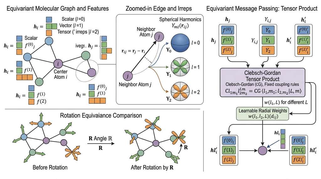
The tensor product is the central operation. Given two irreps of degrees $\ell_1$ and $\ell_2$, their tensor product decomposes into irreps of degrees $|\ell_1 - \ell_2|, \ldots, \ell_1 + \ell_2$ via the Clebsch-Gordan coefficients, where these coefficients are fixed numerical constants (derived from the group's representation theory) that prescribe exactly how two irreps of given degrees combine into each allowed output degree :

$$(\mathbf{u}^{(\ell_1)} \otimes \mathbf{v}^{(\ell_2)})^{(\ell_3)}_m = \sum_{m_1, m_2} C^{\ell_3 m}_{\ell_1 m_1, \ell_2 m_2} \, u^{(\ell_1)}_{m_1} \, v^{(\ell_2)}_{m_2}$$

The Clebsch-Gordan coefficients $C$ are fixed mathematical constants (not learned), which guarantees that the tensor product output transforms correctly under rotations.

A gated nonlinearity is used instead of a standard activation like ReLU because applying ReLU component-wise to a vector or tensor feature would break equivariance; the output would depend on the coordinate system. The gating trick sidesteps this: scalar ($\ell=0$) features pass through a conventional activation, while higher-order ($\ell \geq 1$) features are multiplied by a learned scalar gate, preserving their directional structure.

Mental Model

Think of the Clebsch-Gordan tensor product like mixing paint colors under strict labeling rules. Each input "paint" carries a label describing its type (pure red, pure blue, etc.), and the mixing rules dictate exactly which new labeled colors can result from combining two inputs. Mixing red and yellow always produces orange, never green; the rules are fixed by the color wheel (the group theory), not by the painter (the network weights). The network gets to choose how much of each valid combination to use (the learnable weights), but it can never produce a combination the rules forbid. This is why equivariance is guaranteed: the allowed "color mixtures" (output irreps) are fully determined by the input types, and the fixed coefficients enforce physically consistent transformations regardless of what the network learns.

import torch
from e3nn import o3

# Define irreducible representations
# "0e" = scalar (even parity), "1o" = vector (odd parity), "2e" = rank-2 tensor
irreps_input = o3.Irreps("16x0e + 8x1o + 4x2e")  # 16 scalars, 8 vectors, 4 tensors

# Spherical harmonics for edge features (up to degree 2)
irreps_sh = o3.Irreps.spherical_harmonics(lmax=2)  # "1x0e + 1x1o + 1x2e"

# Tensor product layer: combine node features with edge spherical harmonics
tp = o3.FullyConnectedTensorProduct(
    irreps_in1=irreps_input,      # node features from neighbor
    irreps_in2=irreps_sh,         # edge spherical harmonics
    irreps_out=irreps_input,      # output node features (same type)
)
print(f"Tensor product parameters: {sum(p.numel() for p in tp.parameters()):,}")

# Example: compute message from neighbor to center atom
node_features = torch.randn(1, irreps_input.dim)   # neighbor features
edge_sh = o3.spherical_harmonics(
    irreps_sh, torch.randn(1, 3), normalize=True    # edge direction
)
message = tp(node_features, edge_sh)
print(f"Input dim: {irreps_input.dim}, Output dim: {message.shape[-1]}")

Constructing an e3nn tensor product layer that couples 16 scalar, 8 vector, and 4 rank-2 tensor node features with degree-2 edge spherical harmonics, producing a single equivariant message with internally computed Clebsch-Gordan coefficients and learnable mixing weights.

4. The Architecture Landscape: MACE, NequIP, GemNet, EquiformerV2

Four architectures dominate the current landscape for molecular property prediction. Each makes different trade-offs between expressiveness, computational cost, and accuracy:

NequIP (2022)

The first E(3)-equivariant graph neural network (GNN) for interatomic potentials. NequIP uses equivariant tensor product message passing with features up to $\ell = 2$. Its key contribution was demonstrating that equivariance enables training on as few as 100 molecular configurations while achieving DFT-level accuracy (where density functional theory, or DFT, is the quantum-mechanical simulation method that solves for a molecule's electronic structure from first principles ), a dataset so small that a non-equivariant model would barely begin to learn. NequIP processes two-body interactions (pairs of atoms) and relies on deep message passing (4 to 6 layers) to capture many-body effects indirectly.

MACE (2022)

MACE (Multi-ACE) extends equivariant message passing with higher-order tensor products that explicitly encode many-body interactions. While NequIP captures 3-body effects after two message passing layers, MACE captures them in a single layer through a symmetric contraction (a pooling operation that combines messages from multiple neighbors simultaneously, rather than processing them in pairs, to represent three-body and higher-order atomic interactions within one layer) over multiple neighbors. This makes MACE more expressive per layer, enabling shallower networks (2 layers are typical) that are faster at inference. Section 33.4 uses MACE to build a force field.

GemNet (2021)

GemNet takes a geometric approach: instead of tensor products, it uses invariant geometric features (distances, angles, dihedral angles) to construct messages. This avoids the computational overhead of Clebsch-Gordan tensor products while still capturing many-body interactions through explicit angle and dihedral representations. GemNet-OC (the variant optimized for the Open Catalyst benchmark) was among the first models to reach competitive accuracy for large-scale catalyst screening.

EquiformerV2 (2024)

EquiformerV2 combines equivariant features with the Transformer attention mechanism. The key innovation is equivariant attention: the attention weights are computed from invariant (scalar) features, but they modulate equivariant (vector and tensor) value features. This allows the model to attend to physically relevant interactions while maintaining exact equivariance. As of early 2025, EquiformerV2 achieved leading results on the OC20 and OC22 benchmarks from FairChem, demonstrating that the Transformer architecture scales effectively in the equivariant setting (EquiformerV2 and related catalyst models are available through the fairchem-core package, which supersedes the earlier ocp-models repository).

Practical Example: Choosing an Architecture for Your Problem

A materials science group wants to screen 10,000 candidate catalyst surfaces for CO2 reduction activity. They have DFT calculations for 500 surfaces and need to predict adsorption energies for the rest. Which architecture should they choose?

If accuracy is paramount and compute budget is generous: EquiformerV2 with pre-training on OC20. Transfer learning from the large catalyst dataset dramatically reduces the need for task-specific DFT data.

If inference speed matters (e.g., for molecular dynamics): MACE with 2 layers and $\ell_{\max} = 2$. Its shallow architecture and efficient symmetric contraction make it the fastest among the equivariant models at comparable accuracy.

If the team has limited equivariant ML expertise: GemNet-OC, which avoids the complexity of tensor products and spherical harmonics while still achieving strong results. Its invariant geometric features are more intuitive for domain scientists.

5. Building Equivariant Layers with e3nn

The e3nn library is the foundational toolkit for building equivariant architectures in PyTorch. It provides spherical harmonics, Clebsch-Gordan tensor products, equivariant linear layers, and gated nonlinearities as composable modules (as of 2024, NVIDIA's cuequivariance library offers CUDA-accelerated implementations of key e3nn operations, providing significant speedups for production workloads while maintaining the same API conventions).

Real-World Application: Universal Atomistic Simulation

import torch
from e3nn import o3
from e3nn.nn import FullyConnectedNet, Gate

class EquivariantBlock(torch.nn.Module):
    """One equivariant message-passing layer using e3nn."""

    def __init__(self, irreps_node, irreps_edge_sh, irreps_out):
        super().__init__()
        self.irreps_node = irreps_node

        # Tensor product: combine neighbor features with edge harmonics
        self.tp = o3.FullyConnectedTensorProduct(
            irreps_node, irreps_edge_sh, irreps_out
        )
        # Radial network: scalar weights depending on interatomic distance
        self.radial_net = FullyConnectedNet(
            [1, 64, 64, self.tp.weight_numel],
            act=torch.nn.functional.silu,
        )
        # Gated nonlinearity for equivariant features
        # Scalars use sigmoid gates, higher-order features use norm gates
        irreps_scalars = o3.Irreps(
            [(mul, ir) for mul, ir in irreps_out if ir.l == 0]
        )
        irreps_gated = o3.Irreps(
            [(mul, ir) for mul, ir in irreps_out if ir.l > 0]
        )
        irreps_gates = o3.Irreps(f"{irreps_gated.num_irreps}x0e")

        self.gate = Gate(
            irreps_scalars, [torch.nn.functional.silu] * len(irreps_scalars),
            irreps_gates, [torch.sigmoid] * len(irreps_gates),
            irreps_gated,
        )

    def forward(self, node_features, edge_index, edge_sh, edge_dist):
        """
        node_features: (N, irreps_node.dim) equivariant node features
        edge_index: (2, E) source and target atom indices
        edge_sh: (E, irreps_edge_sh.dim) spherical harmonics of edge vectors
        edge_dist: (E, 1) interatomic distances
        """
        src, dst = edge_index
        neighbor_features = node_features[src]

        # Compute radial weights from distances (invariant)
        radial_weights = self.radial_net(edge_dist)

        # Tensor product with learned radial modulation
        messages = self.tp(neighbor_features, edge_sh, radial_weights)

        # Aggregate messages at each node
        out = torch.zeros_like(node_features[:, :messages.shape[-1]])
        out.index_add_(0, dst, messages)

        # Apply equivariant nonlinearity
        return self.gate(out)

Full equivariant message-passing block with radial-distance-modulated tensor product, index-based neighbor aggregation, and a Gate nonlinearity that applies SiLU to scalar channels and sigmoid-gated norm activations to vector and tensor channels.

Library Shortcut: e3nn + MACE vs. From Scratch

The equivariant block above is approximately 60 lines of code and handles a single message-passing layer. A full equivariant GNN for molecular property prediction (with embedding, multiple layers, readout, and force computation) would be 300 to 500 lines. The MACE repository provides a complete, optimized implementation that includes multi-GPU training, mixed-precision support, pre-trained foundation models, and integration with the Atomic Simulation Environment (ASE) for molecular dynamics. For production use, MACE reduces the implementation from weeks to a single pip install mace-torch and a configuration file.

6. Parity and the O(3) vs. SE(3) Decision

The architectures above all handle rotations and translations, but physical systems have one more geometric symmetry to consider: reflection.

Rotations preserve handedness (chirality), but reflections swap it. This distinction matters because mirror-image molecules (enantiomers) can differ in biological activity. The choice between O(3) equivariance (including reflections) and SE(3) equivariance (rotations and translations only) depends on whether the application must distinguish mirror images:

Use O(3) when predicting properties that are the same for a molecule and its mirror image (energy, heat capacity, density). The e3nn convention labels irreps with parity: "0e" (even scalar), "1o" (odd vector), "2e" (even tensor).
Use SE(3) when predicting properties that differ between enantiomers (optical rotation, biological activity, drug efficacy). Because SE(3) does not include reflections, the network can learn to assign different predictions to a molecule and its mirror image. This requires using pseudoscalar and pseudovector features that change sign under reflection.

Most force field applications use O(3) equivariance because interatomic potentials are parity-invariant. Drug discovery applications may need SE(3) to capture chirality-dependent binding (connecting to the molecular design methods in Chapter 49).

Research Frontier: Scaling Equivariant Models (2024-2026)

The computational cost of tensor products scales as $O(\ell_{\max}^6)$ in the worst case, limiting practical architectures to $\ell_{\max} = 2$ or 3. Recent work addresses this scaling challenge from multiple directions. eSCN (Passaro & Zitnick, 2023) replaces tensor products with equivariant convolutions on the sphere, reducing the cost to $O(\ell_{\max}^3)$. MACE-OFF23 (Kovács et al., 2023) provides a transferable organic force field trained on coupled-cluster-quality data, achieving sub-chemical-accuracy on drug-like molecules without per-system fitting. Equivariant foundation models (MACE-MP-0, JMP-L) pre-trained on millions of DFT calculations from the Materials Project and Alexandria databases are emerging as general-purpose starting points, much as foundation models (Chapter 27) serve as starting points in NLP. Beyond these, MACE-MPA-0 (Batatia et al., 2024) demonstrates that a single universal potential trained on 1.6 million inorganic structures from the Materials Project and Alexandria can achieve near-DFT accuracy across the periodic table without task-specific fine-tuning, establishing a new paradigm where practitioners start from a pre-trained checkpoint rather than training from scratch.

Try It: Verify Equivariance with e3nn

Build and test an equivariant tensor product layer in under 30 minutes using only Python, PyTorch, and the e3nn library.

Step 1. Install the required packages: pip install torch e3nn.

Step 2. Create a tensor product that combines $\ell=1$ vector features with $\ell=1$ spherical harmonics: tp = o3.FullyConnectedTensorProduct("1x1o", "1x1o", "1x0e + 1x1o + 1x2e"). Print the output irreps and confirm the selection rules produce $\ell \in \{0, 1, 2\}$.

Step 3. Generate a random 3D input vector and compute its spherical harmonics with o3.spherical_harmonics. Pass both through the tensor product to get an output.

Step 4. Generate a random rotation matrix using R = o3.rand_matrix(). Rotate both inputs using the appropriate Wigner D-matrices (o3.Irreps("1x1o").D_from_matrix(R)), pass the rotated inputs through the same tensor product, and store the result.

Step 5. Rotate the original output using the D-matrices for the output irreps. Compare the rotated original output with the output from rotated inputs: they should match to floating-point precision (difference below $10^{-5}$). This confirms the layer is exactly equivariant, not approximately so.

Exercise 33.3.1

Consider a tensor product of an $\ell = 1$ (vector) feature with an $\ell = 2$ (rank-2 tensor) feature. Using the Clebsch-Gordan selection rule $|\ell_1 - \ell_2| \leq \ell_3 \leq \ell_1 + \ell_2$, list all output irrep degrees $\ell_3$ that appear. For each, state the dimensionality $(2\ell_3 + 1)$. What is the total dimension of the tensor product output?

Hint

With $\ell_1 = 1$ and $\ell_2 = 2$, the allowed output degrees run from $|1 - 2| = 1$ to $1 + 2 = 3$. Sum up $2\ell_3 + 1$ for each allowed $\ell_3$ to get the total output dimension.

Step-Through: Clebsch-Gordan Tensor Product ($\ell=1 \otimes \ell=1$)

Trace the tensor product of two $\ell = 1$ vectors $\mathbf{u} = (1, 0, 0)$ and $\mathbf{v} = (0, 1, 0)$ into its irrep components.

Step 1. The selection rule gives output degrees $\ell_3 \in \{0, 1, 2\}$.

Step 2 ($\ell_3 = 0$, scalar). The single CG coefficient $C^{00}_{1m_1, 1m_2}$ is nonzero only when $m_1 = -m_2$, yielding the scalar $\frac{1}{\sqrt{3}}(u_{-1}v_1 - u_0 v_0 + u_1 v_{-1})$. For our inputs (converting to the $m = -1, 0, +1$ basis: $u_{+1} = -1/\sqrt{2}$, $u_{-1} = 1/\sqrt{2}$, $u_0 = 0$; $v_{+1} = i/\sqrt{2}$, $v_{-1} = i/\sqrt{2}$, $v_0 = 0$), this evaluates to $\frac{1}{\sqrt{3}} \cdot \frac{i}{\sqrt{2}} \cdot (-1/\sqrt{2} - 1/\sqrt{2}) = -i\sqrt{2/3}$.

Step 3 ($\ell_3 = 1$, vector). The antisymmetric combination gives the cross product $\mathbf{u} \times \mathbf{v} = (0, 0, 1)$, which is indeed a pseudovector (odd parity), consistent with the $1o$ irrep.

Step 4 ($\ell_3 = 2$, tensor). The symmetric traceless combination yields 5 components encoding the quadrupole structure. In Cartesian terms, the traceless part of $u_i v_j + u_j v_i$ has nonzero entries only at $xy$ and $yx$, giving a pure $m = \pm 2$ quadrupole.

The full output is 1 + 3 + 5 = 9 numbers, matching the dimension of $\ell=1 \otimes \ell=1$. Each piece transforms independently under rotation, which is why the network can learn separate weights for each output channel.

Real-World Application: Universal Atomistic Simulation

The MACE-MP-0 foundation model, trained on 150,000 inorganic structures from the Materials Project, powers the matbench-discovery benchmark for crystal stability prediction. Researchers at Microsoft and the University of Cambridge use it as a drop-in replacement for density functional theory in high-throughput screening pipelines, evaluating thousands of candidate battery cathodes and thermoelectric materials per day at a computational cost reported to be roughly 1,000 times lower than running DFT for each structure.

The Hydrogen Atom Knew It All Along

The spherical harmonics that underpin every equivariant neural network were first worked out by Laplace in 1782, over a century before quantum mechanics existed. When Schrödinger solved the hydrogen atom in 1926, the angular part of each electron orbital turned out to be exactly a spherical harmonic: the $s$ orbital is $Y_0^0$, the three $p$ orbitals are $Y_1^{-1}, Y_1^0, Y_1^1$, and the five $d$ orbitals are the $\ell = 2$ harmonics. The mathematics that 18th-century astronomers developed to map gravitational fields on the surface of the Earth is the same mathematics that modern ML architectures use to guarantee rotational equivariance in molecular simulations.

Lab: Equivariance Stress Test

Goal: Empirically verify that an equivariant layer is exactly equivariant while a standard multilayer perceptron (MLP) is not, and measure how equivariance error grows with the number of random rotations for the MLP.

Tools: Python, PyTorch, e3nn (pip install torch e3nn).

Procedure (20 minutes): (1) Build a FullyConnectedTensorProduct("8x1o", "1x1o + 1x2e", "8x0e + 4x1o") layer. (2) Build a plain torch.nn.Linear with matching input and output dimensions. (3) Generate 100 random rotation matrices with o3.rand_matrix(). (4) For each rotation, compute the equivariance error: $\|f(D_{\text{in}} R \cdot x) - D_{\text{out}} R \cdot f(x)\|$ for both models. (5) Plot histograms of the error for both models on the same axes.

What to vary: Try increasing $\ell_{\max}$ from 1 to 3 in the tensor product; observe that the equivariance error stays at machine precision regardless of degree. For the MLP, try adding data augmentation (random rotations during a short training loop) and re-measure: does the error shrink, and does it ever reach machine precision?

What to observe: The tensor product error should stay below $10^{-6}$ (floating-point noise). The MLP error will typically be on the order of $10^{-1}$ to $10^{0}$, confirming that equivariance is a structural guarantee, not an empirical approximation.

Exercises

Conceptual: A standard GNN (e.g., Graph Isomorphism Network or Graph Attention Network) uses scalar features at each node and scalar edge weights. Explain why such a network is automatically invariant to rotations but cannot predict vector quantities (like atomic forces) that are equivariant. What would happen if you tried to predict forces as three scalar outputs from such a network?
Coding: Using e3nn, create a tensor product that combines $\ell = 1$ (vector) node features with $\ell = 1$ (vector) edge spherical harmonics. List all the output irreps produced by this tensor product (which values of $\ell$ appear?). Verify that the output transforms correctly by applying a random rotation to both inputs and checking that the output rotates accordingly.
Analysis: Download the rMD17 aspirin dataset (where rMD17 is a revised version of the MD17 benchmark containing molecular dynamics trajectories recomputed at higher numerical precision , available via torch_geometric.datasets). Train two models: (a) a SchNet model (invariant, uses only distances) and (b) a NequIP-style model (equivariant, uses spherical harmonics). Compare their force mean absolute error (MAE) using the same training set size (950 configurations). By what factor does the equivariant model outperform? How does the gap change if you reduce the training set to 100 configurations?