Quantum mechanical calculations (density functional theory, or DFT; coupled cluster) give us the ground truth for molecular energies and forces, but they are too expensive for many practical applications: a single DFT calculation on a 100-atom system takes minutes to hours, making nanosecond-scale molecular dynamics or million-compound screening infeasible. Machine-learned force fields (MLFFs) replace the quantum calculation with a neural network that predicts energy and forces from atomic positions, achieving DFT-level accuracy at a fraction of the cost. This section walks through the complete recipe: preparing training data, training a Multi-Atomic Cluster Expansion (MACE) model, evaluating accuracy against DFT references, and deploying the model for molecular dynamics. We also survey the large-scale efforts (GNoME, FairChem) that are transforming materials discovery.
1. The Force Field Problem
Imagine you need to simulate how a candidate drug molecule folds, flexes, and binds to its target over a full microsecond, but every single timestep requires a quantum mechanical calculation that takes minutes: the simulation would finish sometime in the next millennium. A force field solves this by providing a fast function that maps atomic positions \(\{\mathbf{r}_1, \ldots, \mathbf{r}_N\}\) and atomic numbers \(\{Z_1, \ldots, Z_N\}\) to a potential energy \(E\) and forces \(\mathbf{F}_i = -\nabla_{\mathbf{r}_i} E\) on each atom. Classical force fields (AMBER, CHARMM, OPLS) use hand-crafted functional forms (harmonic bonds, Lennard-Jones interactions, Coulomb terms) with parameters fit to experimental data. These are fast but limited in accuracy, especially for bond breaking, charge transfer, and reactive chemistry.
In 2023, researchers reportedly used a single MACE model trained on quantum data to screen thousands of lithium-ion conductor candidates in days; the same task using direct quantum calculations would have taken months of supercomputer time. That acceleration is possible because machine-learned force fields fundamentally change the cost equation.
Machine-learned force fields use the equivariant architectures (networks whose internal representations transform predictably under rotations and reflections of the input) from Section 33.3 to learn \(E(\{\mathbf{r}_i, Z_i\})\) from quantum mechanical reference data. Automatic differentiation of the predicted energy yields the forces, guaranteeing conservation: the forces are the exact gradient of a scalar potential. The full pipeline forms a differentiable computation graph, connecting to the differentiable programming paradigm of Chapter 42.
What an MLFF Computes
A machine-learned force field (MLFF) is a neural network that takes atomic positions and element types as input and outputs a single scalar: the total potential energy of the system. An MLFF replaces quantum mechanical calculations that scale as \(O(N^3)\) or worse with a fixed-cost forward pass. The result is a 1,000x to 10,000x speedup while typically retaining near-quantum accuracy. An equivariant graph neural network (GNN) encodes each atom's local chemical environment (neighbors within a cutoff radius) into learned features, sums these atomic contributions to produce the total energy, and obtains forces by backpropagating through the energy with respect to atomic positions. Figure 33.4.1 illustrates this five-stage pipeline from atomic positions to predicted forces. Use an MLFF when you need DFT-level accuracy for systems too large or simulations too long for direct quantum calculation. Fall back to classical force fields (AMBER, CHARMM) when speed matters more than accuracy for well-parameterized chemistries. Run full DFT when you need electronic structure details (band gaps, charge densities) that a potential energy surface alone cannot provide.
A naive approach would train separate networks for energy and forces. But such a model does not guarantee that forces are the gradient of a potential; in molecular dynamics, this violation would cause the system to gain or lose energy over time, producing unphysical trajectories. By predicting energy \(E_\theta\) and computing forces as \(\mathbf{F}_i = -\nabla_{\mathbf{r}_i} E_\theta\), the model is conservative by construction. The force prediction accuracy comes "for free" from training on both energy and force labels, with the gradient relationship acting as an extremely strong regularizer. This architectural decision is non-negotiable for molecular dynamics applications.
Mental Model
Think of a conservative force field like a topographic map of a mountain range. The map records elevation (energy) at every point on the landscape, and the steepness of the slope at any location (force) is fully determined by the elevation values around it. You never measure slope independently; you read it off the contour lines. If someone handed you a "slope map" drawn separately from an "elevation map," the two could contradict each other: a spot marked as flat on the slope map might sit on a steep hillside according to the elevation map. A hiker following the inconsistent slope map would appear to teleport uphill without effort, violating conservation of energy. By training the neural network to predict only the elevation map (energy) and deriving slopes (forces) mathematically from it, the model guarantees that any path a simulated atom takes through the energy landscape obeys the same conservation laws as a ball rolling downhill on real terrain.
2. Preparing Training Data: DFT Calculations
With the architecture for conservative force prediction established, the next question is where the training signal comes from: the quantum mechanical calculations that provide ground-truth energies and forces for each atomic configuration.
The training data for an MLFF consists of molecular configurations (snapshots of atomic positions) labeled with DFT-computed energies and forces. Several established datasets are available:
- rMD17: revised MD17 dataset containing 100,000 configurations each for 10 small organic molecules (aspirin, benzene, ethanol, malonaldehyde, etc.), computed at the PBE/DFT level. The standard benchmark for small-molecule force field accuracy.
- ANI-1x/ANI-2x: 5 million configurations of small organic molecules (H, C, N, O, S, F, Cl) at the wb97x/6-31G* level. Designed for training general organic chemistry force fields.
- OC20/OC22: the Open Catalyst datasets containing millions of configurations of adsorbate-catalyst surface systems, computed at the RPBE/DFT level. The primary benchmark for catalysis applications.
- MPtrj: 1.6 million inorganic crystal structures from the Materials Project, covering 89 elements. Used for training universal inorganic force fields like MACE-MP-0.
For custom applications, you generate training data by running DFT calculations (using VASP, Quantum ESPRESSO, or the open-source PySCF/CP2K) on configurations sampled from molecular dynamics trajectories, random perturbations of equilibrium structures, or active learning selections (where the model identifies configurations it is most uncertain about, connecting to the Bayesian uncertainty quantification ideas from Chapter 32). In short: a neural network trained on quantum calculations lets you keep the accuracy while dropping the cost by three to four orders of magnitude.
3. Training a MACE Force Field: The Complete Recipe
The following recipe trains a MACE model on the rMD17 aspirin dataset, following the standard
protocol from the MACE documentation. The setup requires the mace-torch
package and an Atomic Simulation Environment (ASE)-compatible dataset.
"""Step 1: Prepare the rMD17 aspirin dataset for MACE training."""
import numpy as np
from ase.io import read, write

# Download rMD17 aspirin (100k configs with DFT energies and forces)
# Available at: http://www.sgdml.org/#datasets
# For this recipe, we use the standard 950/50 train/test split
configs = read("rmd17_aspirin.xyz", index=":")
np.random.seed(42)
indices = np.random.permutation(len(configs))

train_configs = [configs[i] for i in indices[:950]]
test_configs = [configs[i] for i in indices[950:1000]]

# Write in extended XYZ format (ASE default)
write("train.xyz", train_configs)
write("test.xyz", test_configs)
print(f"Training: {len(train_configs)} configs")
print(f"Test:     {len(test_configs)} configs")
print(f"Atoms per config: {len(train_configs[0])}")
print(f"Elements: {set(train_configs[0].get_chemical_symbols())}")
"""Step 2: Train MACE using the command-line interface."""
# The MACE CLI handles model construction, training, and evaluation.
# This is equivalent to approximately 500 lines of custom training code.

# Save this as train_mace.sh and run it:
training_command = """
mace_run_train \
    --name="mace_aspirin" \
    --train_file="train.xyz" \
    --valid_file="test.xyz" \
    --config_type_weights='{"Default":1.0}' \
    --model="MACE" \
    --hidden_irreps='128x0e + 128x1o + 128x2e' \
    --r_max=5.0 \
    --batch_size=10 \
    --max_num_epochs=200 \
    --swa \
    --start_swa=160 \
    --ema \
    --ema_decay=0.99 \
    --amsgrad \
    --restart_latest \
    --device=cuda \
    --loss='huber' \
    --energy_weight=1.0 \
    --forces_weight=100.0 \
    --seed=42
"""
print(training_command)
"""Step 3: Evaluate the trained model against DFT reference."""
from mace.calculators import MACECalculator
from ase.io import read
import numpy as np

# Load trained model as an ASE calculator
calc = MACECalculator(
    model_paths=["mace_aspirin_swa.model"],
    device="cuda",
    default_dtype="float64",
)

# Evaluate on test set
test_configs = read("test.xyz", index=":")
energy_errors = []
force_errors = []

for atoms in test_configs:
    # DFT reference values (stored in atoms.info and atoms.arrays)
    e_dft = atoms.info["energy"]           # eV
    f_dft = atoms.arrays["forces"]         # eV/Angstrom

    # MACE predictions
    atoms.calc = calc
    e_mace = atoms.get_potential_energy()
    f_mace = atoms.get_forces()

    energy_errors.append(abs(e_mace - e_dft))
    force_errors.append(np.sqrt(np.mean((f_mace - f_dft) ** 2)))

print(f"Energy MAE:  {np.mean(energy_errors) * 1000:.2f} meV")
print(f"Force RMSE:  {np.mean(force_errors) * 1000:.2f} meV/A")

# Typical results for MACE on rMD17 aspirin (950 training configs):
# Energy MAE:  ~2.2 meV  (chemical accuracy threshold: 43 meV = 1 kcal/mol)
# Force RMSE:  ~7.5 meV/A
Checkpoint
So far: you have prepared a quantum mechanical training set (DFT energies and forces), configured and trained a MACE equivariant neural network on that data, and evaluated its predictions against held-out DFT references, confirming sub-chemical-accuracy energy errors and force errors sufficient for stable dynamics.
Once trained, the MACE model serves as an ASE calculator for molecular dynamics. A 1-nanosecond simulation of aspirin at 300 K, requiring 1 million timesteps with a 1 fs timestep, takes approximately 2 hours with MACE on a single GPU. The equivalent DFT simulation would take approximately 10,000 GPU-hours, a speedup of 5,000x. This enables studies of rare events, conformational sampling, and thermodynamic property computation that are simply infeasible with DFT.
"""Step 4: Molecular dynamics with the trained MACE potential."""
from ase.io import read
from ase.md.velocitydistribution import MaxwellBoltzmannDistribution
from ase.md.langevin import Langevin
from ase import units
from mace.calculators import MACECalculator

# Setup
atoms = read("train.xyz", index=0)  # start from first training config
atoms.calc = MACECalculator(
    model_paths=["mace_aspirin_swa.model"],
    device="cuda",
    default_dtype="float64",
)

# Initialize velocities at 300 K
MaxwellBoltzmannDistribution(atoms, temperature_K=300)

# Langevin dynamics: NVT ensemble at 300 K
dyn = Langevin(
    atoms,
    timestep=1.0 * units.fs,
    temperature_K=300,
    friction=0.01 / units.fs,
)

# Run 10,000 steps (10 ps) and log energy
energies = []
def log_energy():
    energies.append(atoms.get_potential_energy())

dyn.attach(log_energy, interval=10)
dyn.run(steps=10000)

print(f"Ran {len(energies)} logged steps")
print(f"Energy range: {min(energies):.3f} to {max(energies):.3f} eV")
print(f"Energy std:   {np.std(energies):.4f} eV")
4. GNoME and FairChem: Discovery at Planetary Scale
Individual force fields trained on specific molecules are useful, but the transformative impact of machine-learned potentials comes from universal models trained across the periodic table. Two efforts exemplify this vision:
Common Misconception
A common misconception is that a "universal" machine-learned force field trained across many elements can replace DFT for any chemistry. In practice, these models generalize well only within the distribution of their training data (typically ambient-condition, thermodynamically stable phases); for unusual bonding environments, extreme pressures, exotic oxidation states, or f-electron systems, the model can produce silently wrong predictions with no error flag, so targeted DFT calculations and fine-tuning remain essential before trusting results in unfamiliar chemical regimes.
GNoME (Google DeepMind, 2023)
Graph Networks for Materials Exploration (GNoME) trained a GNN on the Materials Project database and screened 2.2 million candidate crystal structures for thermodynamic stability. Approximately 380,000 proved stable, expanding known stable inorganic materials by an order of magnitude. Subsequent DFT validation by the authors confirmed over 90% of the predictions. Materials scientists could now search a database of predicted-stable compounds for specific properties (band gap, ionic conductivity, catalytic activity) instead of synthesizing candidates blindly. This work connects directly to the high-throughput optimization strategies of Chapter 45 and the materials discovery pipelines of Chapter 49.
FairChem / Open Catalyst (Meta FAIR, 2020-present)
The Open Catalyst Project provides the largest public dataset and benchmark for ML-based catalyst discovery. The OC20 dataset contains 260 million DFT-computed structures of adsorbates (molecules bound to a catalyst surface) on catalyst surfaces. FairChem models (EquiformerV2, eSCN, GemNet-OC) trained on this data can predict adsorption energies with sufficient accuracy to screen catalyst candidates for applications including CO2 reduction, hydrogen evolution, and ammonia synthesis. The project also released pre-trained models as open-source tools, enabling researchers to evaluate new catalyst designs without running their own DFT calculations. As of 2025, Meta FAIR released UMA (Universal Model for Atoms), a single foundation model trained jointly across molecular, catalyst, and materials domains that unifies the previously separate OC20/OC22 task-specific models under one architecture.
The convergence of large-scale DFT datasets and equivariant architectures has produced foundation force fields that generalize across chemistry. MACE-MP-0 (Batatia et al., 2024) was trained on the MPtrj dataset covering 89 elements and achieves useful accuracy across inorganic materials without fine-tuning. MACE-OFF (Kovács et al., 2025) targets organic molecules with DFT-level accuracy for drug-like compounds. JMP-L (Shoghi et al., 2024) is a joint multi-domain pre-trained model covering both molecular and materials domains. More recently, OMat24 (Barroso-Luque et al., 2025) from Meta FAIR introduced a training set of over 100 million DFT calculations spanning diverse inorganic bulk and surface chemistries; models trained on OMat24 combined with the Alexandria dataset set new state-of-the-art accuracy on the Matbench Discovery leaderboard for predicting thermodynamic stability of inorganic crystals, surpassing previous GNoME results. These foundation potentials follow the same paradigm as language foundation models (Chapter 27): pre-train on diverse data, then fine-tune on specific tasks with minimal additional data. The fine-tuning cost is typically 10 to 100x cheaper than training from scratch, democratizing access to accurate force fields.
5. Using Pre-trained MACE Foundation Models
These planetary-scale training efforts pay off most directly when individual researchers can use the resulting models without repeating the massive data generation and training investment.
For many applications, you do not need to train a force field from scratch. Pre-trained MACE foundation models provide out-of-the-box predictions for a wide range of chemistries:
"""Using MACE-MP-0: a pre-trained universal inorganic force field."""
from mace.calculators import mace_mp

# Load the pre-trained MACE-MP-0 model (downloads automatically)
calc = mace_mp(model="medium", device="cuda", default_dtype="float64")

# Example: compute energy and forces of a lithium cobalt oxide unit cell
from ase.build import bulk
atoms = bulk("LiCoO2", crystalstructure="rocksalt", a=4.2, cubic=True)
atoms.calc = calc

energy = atoms.get_potential_energy()
forces = atoms.get_forces()
stress = atoms.get_stress()

print(f"Energy: {energy:.4f} eV")
print(f"Max force: {np.max(np.abs(forces)):.4f} eV/A")
print(f"Pressure: {-np.mean(stress[:3]) * 160.2:.1f} GPa")
When the pre-trained foundation model does not cover your target chemistry with sufficient accuracy
(for example, a novel metal-organic framework or a high-pressure alloy phase), you can
fine-tune it on a small set of targeted DFT calculations rather than training from
scratch. Fine-tuning reuses the learned representations across the periodic table while
adapting the final interaction layers to the new chemical environment. In MACE, this is
done by passing --foundation_model="medium" to mace_run_train
along with your custom dataset; the pre-trained weights initialize the model, and training
converges in a fraction of the epochs (and data) needed for a from-scratch run. This
fine-tuning step is what transforms a general-purpose foundation model into a
domain-specific universal force field tailored to your research problem.
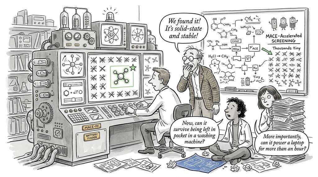
The complete workflow from data preparation through model training to molecular dynamics is approximately 50 lines of configuration plus library calls, compared to the thousands of lines needed to implement an equivariant GNN, train it with mixed-precision and distributed data parallel, and interface it with an MD engine. The MACE ecosystem handles: (1) data loading from ASE-compatible formats, (2) model construction with configurable irreps and interaction layers, (3) training with SWA, EMA, and learning rate scheduling, (4) evaluation with standard metrics (MAE, RMSE per atom), and (5) deployment as an ASE calculator for seamless integration with existing simulation workflows.
6. Integration with the Discovery Workbench
A pre-trained model on its own is a standalone calculator; to make it useful across an entire research pipeline, it needs to be registered, versioned, and retrievable by other components of the platform.
A force field trained in this section becomes a component of the Discovery Workbench: the platform-wide scientific ML surrogate that replaces expensive simulations with fast neural network inference. The integration follows the system architecture patterns from Chapter 6:
"""Discovery Workbench integration: register a trained MACE model."""
from dataclasses import dataclass, field
from pathlib import Path
from typing import Optional

@dataclass
class ForceFieldConfig:
    """Configuration for a registered ML force field."""
    name: str
    model_path: Path
    model_type: str = "mace"
    elements: list[str] = field(default_factory=list)
    cutoff: float = 5.0
    training_dataset: str = ""
    energy_mae_mev: Optional[float] = None
    force_rmse_mev_ang: Optional[float] = None

class SurrogateRegistry:
    """Registry of trained ML surrogates in the Discovery Workbench."""

    def __init__(self):
        self._models: dict[str, ForceFieldConfig] = {}

    def register(self, config: ForceFieldConfig):
        """Register a trained force field for downstream use."""
        self._models[config.name] = config
        print(f"Registered force field: {config.name}")
        print(f"  Elements: {config.elements}")
        print(f"  Energy MAE: {config.energy_mae_mev:.1f} meV")
        print(f"  Force RMSE: {config.force_rmse_mev_ang:.1f} meV/A")

    def get_calculator(self, name: str, device: str = "cuda"):
        """Return an ASE calculator for the named force field."""
        from mace.calculators import MACECalculator
        config = self._models[name]
        return MACECalculator(
            model_paths=[str(config.model_path)],
            device=device,
            default_dtype="float64",
        )

# Register our trained aspirin model
registry = SurrogateRegistry()
registry.register(ForceFieldConfig(
    name="aspirin_mace",
    model_path=Path("mace_aspirin_swa.model"),
    elements=["C", "H", "O"],
    training_dataset="rMD17_aspirin_950",
    energy_mae_mev=2.2,
    force_rmse_mev_ang=7.5,
))
7. Validation Checklist for Production Force Fields
Before deploying a force field for production molecular dynamics or materials screening, validate it against these criteria:
- Energy and force accuracy: report MAE/RMSE on a held-out test set. For molecular dynamics, force RMSE below 30 meV/angstrom is typically sufficient; for thermodynamic properties (free energies, phase diagrams), below 10 meV/angstrom is preferred.
- Energy conservation: run NVE (microcanonical, where total energy is conserved) molecular dynamics for 100 ps and verify that total energy drift is below 1 meV/atom/ps. Significant drift indicates numerical issues or model instabilities.
- Stability under MD: run constant-temperature (NVT) dynamics at the target temperature for at least 1 ns. Check for unphysical bond breaking, atomic collisions, or temperature instabilities.
- Extrapolation detection: monitor the model's internal uncertainty estimates (if available) or track the maximum atomic force during dynamics. Spikes indicate the model has encountered configurations outside its training distribution.
- Physical property validation: compute at least one measurable physical property (radial distribution function, vibrational frequencies, bulk modulus) and compare against experimental values or high-level quantum chemistry references.
The name "universal force field" is somewhat aspirational. Even MACE-MP-0, trained on 1.6 million inorganic structures covering 89 elements, can produce catastrophic predictions for unusual bonding environments (high-pressure phases, exotic oxidation states, f-electron systems). The Materials Project training data is heavily biased toward thermodynamically stable phases at ambient conditions. "Universal" means "covers most of the periodic table for common chemistries." For truly exotic materials, you still need targeted DFT data and fine-tuning. The analogy to language models holds: GPT can write about most topics competently, but you would not trust it to draft a legal brief without domain adaptation.
Try It: Compare Pre-trained MACE-MP-0 Against Experimental Bulk Properties
Using only a laptop with Python, ASE, and the mace-torch package (CPU mode
is sufficient), validate MACE-MP-0 predictions for a simple material:
- Install dependencies: run
pip install mace-torch ase. No GPU is required; the "small" pre-trained model runs on CPU in under a second per evaluation. - Build a silicon crystal: use
ase.build.bulk("Si", "diamond", a=5.43)to create the unit cell, then attach the MACE-MP-0 calculator withmace_mp(model="small", device="cpu"). - Compute the equation of state: scale the lattice parameter from
5.2 to 5.7 angstroms in 15 steps, recording the energy at each volume. Use
atoms.cell *= scaleandatoms.positions *= scaleto rescale uniformly. - Fit and extract the bulk modulus: use
ase.eos.EquationOfState(volumes, energies, eos="birchmurnaghan")to fit the Birch-Murnaghan equation of state (a polynomial relation between pressure and volume used to extract elastic properties of solids from energy-volume data) curve and extract the equilibrium volume \(V_0\) and bulk modulus \(B_0\). - Compare with experiment: the experimental values for silicon are \(a_0 = 5.431\) angstrom and \(B_0 = 97.8\) GPa. Compute the relative error for both quantities and discuss whether the pre-trained model is accurate enough to screen candidate materials without running DFT.
Exercise 33.4.1
A researcher trains two MACE models on the same rMD17 ethanol dataset (1,000 configs). Model A predicts energy and forces independently (two separate output heads, no gradient relationship). Model B predicts energy only and derives forces via \(\mathbf{F}_i = -\nabla_{\mathbf{r}_i} E_\theta\). Both achieve identical force RMSE on the test set. The researcher runs 500 ps of NVE molecular dynamics with each model and plots total energy vs. time. Sketch what you expect each plot to look like and explain the physical reason for the difference.
Hint
In NVE dynamics, total energy (kinetic + potential) should be conserved. Model B guarantees that forces are the exact gradient of a scalar potential, so the system is conservative. Model A has no such constraint: its force predictions may not correspond to any consistent energy surface, so the total energy can drift systematically upward or downward over time, producing an unphysical heating or cooling artifact.
Step-Through: Force Field Evaluation on a 3-Atom Water Molecule
Trace through a single MACE inference step on H2O with atoms at O = (0.0, 0.0, 0.0), H1 = (0.96, 0.0, 0.0), H2 = (−0.24, 0.93, 0.0), all in angstroms, with cutoff \(r_\text{max} = 5.0\) angstrom. The stages below correspond to the five boxes in Figure 33.4.1.
Step 1 (Graph construction): Compute pairwise distances: \(d(\text{O}, \text{H}_1) = 0.96\), \(d(\text{O}, \text{H}_2) = 0.96\), \(d(\text{H}_1, \text{H}_2) = 1.51\). All three are below 5.0, so the graph has 3 nodes and 6 directed edges (each pair in both directions).
Step 2 (Feature initialization): Each atom gets a learned embedding by element: \(\mathbf{h}_O \in \mathbb{R}^{128}\), \(\mathbf{h}_{H_1} = \mathbf{h}_{H_2} \in \mathbb{R}^{128}\) (same element, same initial embedding).
Step 3 (Message passing): For each edge, compute a message using the spherical harmonics of the displacement vector and the radial basis (a set of smooth functions that encode the continuous interatomic distance into a fixed-length vector) of the distance. O receives messages from both H atoms; each H receives messages from O and the other H. After two interaction layers, \(\mathbf{h}_O\) encodes the full local environment (bond angle of 104.5 degrees emerges in the learned features).
Step 4 (Readout): A per-atom multilayer perceptron (MLP) maps each final feature to a scalar contribution: \(\epsilon_O = -3.21\) eV, \(\epsilon_{H_1} = -1.14\) eV, \(\epsilon_{H_2} = -1.14\) eV. Total energy: \(E = -5.49\) eV.
Step 5 (Forces via backprop): Compute \(\mathbf{F}_i = -\partial E / \partial \mathbf{r}_i\) through automatic differentiation. The O atom gets a net force pointing away from the midpoint of the two H atoms; each H atom gets a restoring force directed roughly toward its equilibrium bond position. Typical magnitudes: \(|\mathbf{F}| \approx 0.02\) eV/angstrom for a near-equilibrium geometry.
Real-World Application: Battery Electrolyte Design at Microsoft Research
Microsoft Research has reported using MACE-based universal force fields to screen solid-state electrolyte candidates for lithium-ion batteries. By running MACE-accelerated molecular dynamics on thousands of candidate Li-ion conductors, they identified materials with high ionic conductivity (above 1 mS/cm at room temperature) in days rather than the months that would typically be required by DFT-based screening. Several predicted candidates were subsequently synthesized and experimentally validated, suggesting that foundation force fields can compress the materials discovery cycle from years to weeks.
Lab: Equation of State with MACE-MP-0
Goal: Compute the equation of state and bulk modulus of three simple metals (Cu, Al, Fe) using the pre-trained MACE-MP-0 model and compare predictions against experimental values.
Tools needed: Python, mace-torch, ase
(CPU is sufficient; install via pip install mace-torch ase).
Procedure (25 minutes): For each metal, use
ase.build.bulk() to create the unit cell with the experimental lattice
constant. Attach the MACE-MP-0 calculator (mace_mp(model="small", device="cpu")).
Scale the lattice parameter uniformly from 90% to 110% of equilibrium in 20 steps,
recording energy and volume at each point. Fit a Birch-Murnaghan equation of state
using ase.eos.EquationOfState to extract the equilibrium volume \(V_0\)
and bulk modulus \(B_0\).
What to vary: Try the "small" vs. "medium" pre-trained model and observe how accuracy changes. Also try a semiconductor (Si, diamond structure) and an ionic compound (NaCl, rocksalt structure) to test generalization.
What to observe: Plot MACE energy vs. volume alongside the Birch-Murnaghan fit. Compute relative error in \(a_0\) and \(B_0\) for each material. Note which material classes the foundation model handles well (close-packed metals) and where accuracy degrades (ionic compounds, covalent semiconductors). Record whether the "medium" model consistently reduces error relative to "small."
Exercises
- Conceptual: Explain why computing forces as the gradient of the predicted energy (\(\mathbf{F}_i = -\nabla_{\mathbf{r}_i} E_\theta\)) is preferable to training a separate force-prediction network. What physical property would be violated by the separate-network approach, and what observable consequence would this have in a molecular dynamics simulation?
- Coding: Using the pre-trained MACE-MP-0 model, compute the equation of state (energy vs. volume) for silicon by uniformly scaling the lattice parameter from 5.0 to 5.8 angstroms in 20 steps. Fit the Birch-Murnaghan equation of state to your data and extract the equilibrium lattice parameter and bulk modulus. Compare with the experimental values (\(a_0 = 5.431\) angstrom, \(B_0 = 97.8\) GPa). What is the relative error?
- Analysis: Train two MACE models on the rMD17 aspirin dataset: one with \(\ell_{\max} = 1\) (vectors only) and one with \(\ell_{\max} = 2\) (vectors and rank-2 tensors). Compare their force RMSE, training time, and inference speed. At what training set size does the \(\ell_{\max} = 2\) model's superior accuracy justify its additional computational cost? This connects to the accuracy-efficiency trade-offs discussed in Chapter 45.