42.1 Automatic Differentiation

1. Why Not Finite Differences?

The simplest way to estimate a derivative is the finite difference approximation:

where \(e_i\) is the \(i\)-th unit vector and \(h\) is a small step size. This works, but it has two fundamental problems. First, computing the full gradient of \(f: \mathbb{R}^n \to \mathbb{R}\) requires \(n+1\) function evaluations. For a force field with thousands of parameters or a neural network with millions, this cost is prohibitive. Second, the approximation is inherently noisy: too large an \(h\) introduces truncation error, while too small an \(h\) amplifies floating-point rounding error. The sweet spot depends on both the function and the arithmetic precision, making finite differences unreliable for sensitive scientific computations.

Automatic differentiation eliminates both problems. It computes exact derivatives (to machine precision) and, in reverse mode, computes the full gradient in time proportional to a small constant multiple of the original function evaluation, regardless of \(n\). In short: AD turns the chain rule into a compiler pass, delivering exact gradients as a by-product of running the program itself.

What AD Is and When to Use It

When a satellite drag model needs recalibrating, engineers must compute the gradient of a trajectory mismatch with respect to hundreds of atmospheric coefficients; doing this by finite differences means re-running the entire orbit propagation once per coefficient, turning a feasible overnight job into one that would take weeks. Automatic differentiation collapses that cost to a single backward pass.

Automatic differentiation (AD) computes derivatives of numerical programs by decomposing them into elementary operations (addition, multiplication, \(\sin\), \(\exp\)) and applying the chain rule to each operation in turn. Among general-purpose differentiation strategies, AD is unique in simultaneously delivering machine-precision derivatives and bounded computational overhead. This combination makes AD the backbone of gradient-based optimization in machine learning, scientific simulation, and engineering design. The core mechanism augments every floating-point operation with a companion derivative operation, computing the derivative as a by-product of the original execution. Prefer AD over symbolic differentiation when a function is defined as code rather than a closed-form expression. Prefer it over finite differences when precision matters or when the input dimension makes per-component perturbation expensive.

2. Forward Mode: Dual Numbers and JVPs

Forward-mode AD propagates derivatives alongside values through a computation. The key abstraction is the dual number: a pair \((v, \dot{v})\) where \(v\) is the primal value (the original quantity being computed) and \(\dot{v}\) is the tangent (derivative with respect to some input). Every elementary operation lifts naturally to dual numbers. For addition:

For multiplication:

These rules are just the familiar product rule and sum rule of calculus, applied mechanically. By seeding one input \(x_i\) with tangent \(\dot{x}_i = 1\) and all other inputs with tangent \(0\), a single forward pass produces both the function value and the partial derivative \(\partial f / \partial x_i\).

Let us implement this from scratch, without any AD library, to expose the mechanism.

import math

class Dual:
    """A dual number (value, tangent) for forward-mode AD."""

    def __init__(self, value: float, tangent: float = 0.0):
        self.value = value
        self.tangent = tangent

    def __add__(self, other):
        other = other if isinstance(other, Dual) else Dual(other)
        return Dual(self.value + other.value,
                    self.tangent + other.tangent)

    def __radd__(self, other):
        return Dual(other).__add__(self)

    def __mul__(self, other):
        other = other if isinstance(other, Dual) else Dual(other)
        return Dual(self.value * other.value,
                    self.value * other.tangent + self.tangent * other.value)

    def __rmul__(self, other):
        return Dual(other).__mul__(self)

    def __sub__(self, other):
        other = other if isinstance(other, Dual) else Dual(other)
        return Dual(self.value - other.value,
                    self.tangent - other.tangent)

    def __rsub__(self, other):
        return Dual(other).__sub__(self)

    def __truediv__(self, other):
        other = other if isinstance(other, Dual) else Dual(other)
        return Dual(
            self.value / other.value,
            (self.tangent * other.value - self.value * other.tangent)
                / (other.value ** 2)
        )

    def __pow__(self, n):
        # Only integer/float exponents for simplicity
        return Dual(self.value ** n,
                    n * self.value ** (n - 1) * self.tangent)

    def __repr__(self):
        return f"Dual({self.value}, {self.tangent})"


def dual_sin(x: Dual) -> Dual:
    return Dual(math.sin(x.value), math.cos(x.value) * x.tangent)

def dual_exp(x: Dual) -> Dual:
    e = math.exp(x.value)
    return Dual(e, e * x.tangent)


# Example: f(x) = sin(x^2) * exp(x) at x = 1.5
# Seed x with tangent = 1 to get df/dx
x = Dual(1.5, 1.0)
result = dual_sin(x ** 2) * dual_exp(x)

print(f"f(1.5)  = {result.value:.10f}")
print(f"f'(1.5) = {result.tangent:.10f}")

# Verify against finite differences
import numpy as np
h = 1e-7
f = lambda x: np.sin(x**2) * np.exp(x)
fd_deriv = (f(1.5 + h) - f(1.5)) / h
print(f"f'(1.5) [finite diff] = {fd_deriv:.10f}")
# Output:
# f(1.5)  = 4.2890498995
# f'(1.5) = -6.5578889413
# f'(1.5) [finite diff] = -6.5578886498

The dual number approach computes a Jacobian-vector product (JVP), where the Jacobian \(J \in \mathbb{R}^{m \times n}\) is the matrix of all partial derivatives of a function \(f: \mathbb{R}^n \to \mathbb{R}^m\) (each entry \(J_{ij} = \partial f_i / \partial x_j\)). Seeding the input with a tangent vector \(\dot{x} \in \mathbb{R}^n\) produces \(J \dot{x} \in \mathbb{R}^m\): the directional derivative along \(\dot{x}\). One forward pass computes one column of the Jacobian (by setting \(\dot{x} = e_i\)). For a function with \(n\) inputs and \(m\) outputs, computing the full Jacobian requires \(n\) forward passes. This makes forward mode efficient when \(n\) is small (few inputs, many outputs).

3. Reverse Mode: Adjoints and VJPs

Reverse-mode AD is the algorithm behind backpropagation. Where forward mode propagates tangents from inputs to outputs, reverse mode propagates adjoints (also called cotangents or sensitivities; "cotangent" because the adjoint lives in the dual vector space of the output, mapping output perturbations back to input sensitivities) from outputs back to inputs. An adjoint \(\bar{v}\) of an intermediate variable \(v\) represents the derivative of the final output with respect to \(v\) (that is, \(\bar{v} = \partial L / \partial v\) for a scalar loss \(L\)). The key operation is the vector-Jacobian product (VJP): given an adjoint vector \(\bar{y} \in \mathbb{R}^m\) at the output, reverse mode computes \(\bar{x} = J^T \bar{y} \in \mathbb{R}^n\), which is the gradient of a scalar loss \(L = \bar{y}^T f(x)\) with respect to all \(n\) inputs.

Critically, one reverse pass computes one row of \(J^T\) (equivalently, one row of the full gradient). For a scalar-valued function \(f: \mathbb{R}^n \to \mathbb{R}\), a single reverse pass produces the entire gradient \(\nabla f \in \mathbb{R}^n\). This is why training a neural network with millions of parameters is feasible: in practice, the gradient computation typically costs roughly 2 to 4 times the forward pass, regardless of parameter count.

To implement reverse mode, we record a computational graph (the "tape," a data structure that logs each operation and its inputs during the forward pass so the backward pass can retrace them) during the forward pass, then walk it backwards accumulating adjoints. Here is a minimal implementation:

class Var:
    """A traced variable for reverse-mode AD."""

    def __init__(self, value: float, children=(), grad_fns=()):
        self.value = value
        self.children = children      # parent Var nodes
        self.grad_fns = grad_fns      # one function per child
        self.grad = 0.0               # accumulated adjoint

    def __add__(self, other):
        other = other if isinstance(other, Var) else Var(other)
        return Var(self.value + other.value,
                   children=(self, other),
                   grad_fns=(lambda g: g, lambda g: g))

    def __mul__(self, other):
        other = other if isinstance(other, Var) else Var(other)
        # Capture values for the backward pass
        sv, ov = self.value, other.value
        return Var(self.value * other.value,
                   children=(self, other),
                   grad_fns=(lambda g, o=ov: g * o,
                             lambda g, s=sv: g * s))

    def __sub__(self, other):
        other = other if isinstance(other, Var) else Var(other)
        return Var(self.value - other.value,
                   children=(self, other),
                   grad_fns=(lambda g: g, lambda g: -g))

    def __pow__(self, n):
        v = self.value
        return Var(v ** n,
                   children=(self,),
                   grad_fns=(lambda g, v=v, n=n: g * n * v ** (n - 1),))

    def __radd__(self, other):
        return Var(other).__add__(self)

    def __rmul__(self, other):
        return Var(other).__mul__(self)

    def backward(self):
        """Reverse-mode sweep: accumulate adjoints via topological order."""
        topo_order = []
        visited = set()

        def build_topo(node):
            if id(node) not in visited:
                visited.add(id(node))
                for child in node.children:
                    build_topo(child)
                topo_order.append(node)

        build_topo(self)
        self.grad = 1.0  # seed: dL/dL = 1

        for node in reversed(topo_order):
            for child, grad_fn in zip(node.children, node.grad_fns):
                child.grad += grad_fn(node.grad)


# Example: f(x, y) = (x*y + x^2) at x=3, y=4
# Analytic: df/dx = y + 2x = 10, df/dy = x = 3
x = Var(3.0)
y = Var(4.0)
z = x * y + x ** 2
z.backward()

print(f"f(3, 4) = {z.value}")    # 24.0
print(f"df/dx   = {x.grad}")     # 10.0
print(f"df/dy   = {y.grad}")     # 3.0

4. Forward vs. Reverse: The Cost Calculus

The computational cost of AD depends on the shape of the Jacobian. Consider a function \(f: \mathbb{R}^n \to \mathbb{R}^m\) with Jacobian \(J \in \mathbb{R}^{m \times n}\).

• Forward mode computes one column of \(J\) per pass (one JVP). Cost for the full Jacobian: \(O(n)\) forward passes.
• Reverse mode computes one row of \(J\) per pass (one VJP). Cost for the full Jacobian: \(O(m)\) reverse passes.

The rule of thumb: use forward mode when \(n \ll m\) (few inputs, many outputs) and reverse mode when \(m \ll n\) (few outputs, many inputs). For the dominant use case in scientific discovery, computing the gradient of a scalar loss with respect to many parameters (\(m = 1\), \(n\) large), reverse mode wins decisively. This is why backpropagation (reverse-mode AD) is the workhorse of deep learning and differentiable simulation.

When both \(n\) and \(m\) are large, neither mode alone is optimal for the full Jacobian. Mixed-mode AD (which selects forward mode along dimensions where \(n\) is smaller and reverse mode where \(m\) is smaller) computes the Jacobian in \(\min(n, m)\) passes by choosing the cheaper direction for each block. JAX supports both modes seamlessly: jax.jvp for forward mode and jax.grad (built on jax.vjp) for reverse mode.

5. The Computational Graph Perspective

Both forward and reverse mode can be understood through the lens of computational graphs. Consider a function decomposed into elementary operations:

The chain rule gives:

Forward mode evaluates this product left-to-right (from inputs toward outputs). Reverse mode evaluates it right-to-left (from outputs toward inputs). Neither mode forms the intermediate Jacobians explicitly; instead, each mode accumulates matrix-vector products one factor at a time. Figure 42.1 illustrates this distinction on a small computational graph for \(f(x, y) = (x + y) \cdot x\). Figure 42.1.1 illustrates forward-mode vs reverse-mode AD on a computational graph.

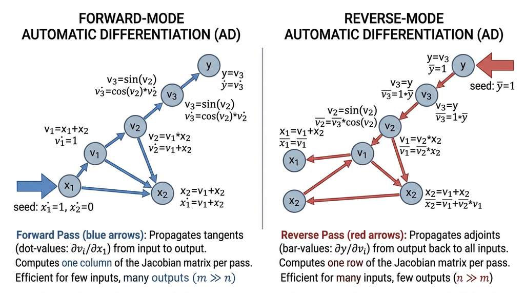
For a chain of \(k\) operations each with Jacobian of size \(d \times d\), both modes cost \(O(k d^2)\) to evaluate the full Jacobian. The difference appears when the dimensions are not uniform: reverse mode shines for "fan-in" graphs (many inputs converge to one output), while forward mode shines for "fan-out" graphs (one input diverges to many outputs).

Beyond first-order gradients, many scientific applications require curvature information to distinguish saddle points from minima or to accelerate convergence, and AD provides an elegant route to these higher-order quantities.

6. Higher-Order Derivatives

AD modes compose. Computing a Hessian-vector product \(H v = \nabla^2 f \cdot v\) (where \(H = \nabla^2 f\) is the Hessian, the matrix of second partial derivatives with entry \(H_{ij} = \partial^2 f / \partial x_i \partial x_j\)) can be done by applying forward mode to a reverse-mode gradient computation. Concretely, if \(g(x) = \nabla f(x)\) is computed by reverse mode, then a forward-mode JVP of \(g\) along direction \(v\) gives \(Hv\). This costs roughly twice a gradient evaluation, regardless of dimension, and never forms the full \(n \times n\) Hessian matrix.

import jax
import jax.numpy as jnp

def rosenbrock(xy):
    """Rosenbrock function: a classic optimization test case."""
    x, y = xy
    return (1.0 - x) ** 2 + 100.0 * (y - x ** 2) ** 2

# Gradient (reverse mode)
grad_fn = jax.grad(rosenbrock)

# Hessian-vector product (forward-over-reverse)
def hvp(f, x, v):
    """Hessian-vector product via forward-over-reverse mode."""
    return jax.jvp(jax.grad(f), (x,), (v,))[1]

x0 = jnp.array([1.0, 1.0])
v = jnp.array([1.0, 0.0])

print(f"Gradient at (1,1): {grad_fn(x0)}")
print(f"Hessian-vector product H @ [1,0]: {hvp(rosenbrock, x0, v)}")

# Full Hessian (for comparison; expensive for large n)
hessian_fn = jax.hessian(rosenbrock)
H = hessian_fn(x0)
print(f"Full Hessian:\n{H}")
print(f"H @ [1,0] directly: {H @ v}")
# Output:
# Gradient at (1,1): [0. 0.]
# Hessian-vector product H @ [1,0]: [802. -400.]
# Full Hessian:
# [[ 802. -400.]
#  [-400.  200.]]
# H @ [1,0] directly: [802. -400.]

7. Checkpointing and Memory Trade-offs

Reverse-mode AD must store intermediate values from the forward pass to use during the backward pass. For a computation with \(k\) steps, this requires \(O(k)\) memory. In a long simulation (thousands of time steps), this can exhaust graphics processing unit (GPU) memory. The standard solution is gradient checkpointing (also called rematerialization): store only a subset of intermediate values, then recompute the others during the backward pass.

With \(\sqrt{k}\) checkpoints evenly spaced through the computation, the memory cost drops to \(O(\sqrt{k})\) at the expense of roughly one additional forward pass. This trade-off is formalized by the revolve algorithm (Griewank, 1992, with the optimal binomial checkpointing schedule, so called because the number of recomputations follows binomial coefficients that minimize total work for a given memory budget; Griewank and Walther published the revolve implementation as ACM Algorithm 799 in 2000). JAX supports checkpointing through jax.checkpoint (also called jax.remat):

import jax

@jax.checkpoint
def expensive_layer(x, params):
    """A computation whose intermediates are not stored during
    the forward pass; they are recomputed during backprop."""
    for w in params:
        x = jax.nn.relu(x @ w)
    return x

# When used inside a jax.grad computation, this layer's
# intermediates are recomputed rather than stored, reducing
# peak memory from O(num_layers * layer_size) to O(layer_size).

Checkpointing becomes critical in Section 42.3 when we backpropagate through molecular dynamics trajectories with thousands of time steps. The adjoint method we derive there provides an even more memory-efficient alternative for ordinary differential equation (ODE)-constrained problems.

With the core algorithms and their memory management strategies established, the remaining question is how real-world software systems implement these ideas in practice.

8. AD in the Wild: Systems and Trade-offs

Modern AD systems fall into two broad categories. Operator overloading systems (PyTorch, our Var class) build the computational graph dynamically during execution. They handle control flow (if/else, while loops) naturally because the graph reflects the specific execution path taken. Source transformation systems (Tapenade, some modes of JAX) analyze the program structure ahead of time and generate derivative code. They can optimize across operations but struggle with data-dependent control flow.

JAX occupies a middle ground: it traces Python functions into a functional representation (an XLA High-Level Operations (HLO) graph) and differentiates that graph. This design combines the cross-operation optimization of source transformation with Python control flow support via jax.lax.cond and jax.lax.scan. The trade-off is a functional constraint (no side effects, no in-place mutation) that pays dividends when we stack transforms in Section 42.2.