33.1 Physics-Informed Neural Networks

1. The Core PINN Idea

In 2017, engineers modeling heat dissipation in a novel battery geometry spent weeks generating a computational mesh before a single simulation could run. Physics-informed neural networks eliminate that bottleneck entirely, replacing grid generation with gradient descent.

Imagine handing a neural network not a labeled dataset but a differential equation, then asking it to find a function whose derivatives satisfy that equation at every point in the domain: no grid, no mesh, no time-stepping loop, just an optimization problem. To see how this works, consider a general PDE defined on a domain \(\Omega \subset \mathbb{R}^d\) with boundary \(\partial\Omega\):

Here \(u(x)\) is the unknown solution, \(\mathcal{N}\) is a (possibly nonlinear) differential operator, \(\mathcal{B}\) is a boundary operator, and \(f, g\) are known source and boundary data. A PINN approximates \(u\) with a neural network \(u_\theta(x)\) parameterized by weights \(\theta\), and trains by minimizing a composite loss:

The three terms serve distinct purposes. The residual loss \(\mathcal{L}_r\) penalizes violations of the PDE at a set of collocation points \(\{x_r^{(i)}\}\) sampled inside the domain:

Collocation points are specific locations in the domain where the PINN evaluates whether the PDE holds. The network cannot check the equation at every point in a continuous domain. Instead, it samples a finite set of locations, penalizes PDE violations there, and relies on its own smoothness to interpolate correct behavior between samples. Unlike grid points in finite-difference methods, you place collocation points randomly, quasi-randomly, or adaptively in regions of large residual. Use random or quasi-random collocation when the solution is smooth across the domain. Switch to adaptive residual-based refinement (adding points where the PDE error is highest) when the solution has localized features such as boundary layers or sharp gradients.

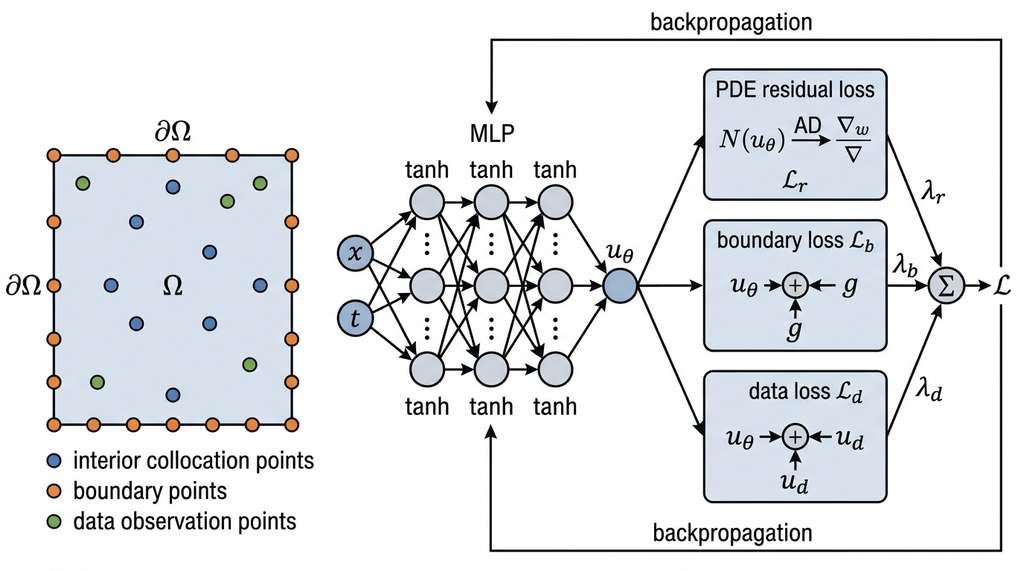
The diagram in Figure 33.1 shows the full PINN training loop: spatial and temporal coordinates enter the network, automatic differentiation computes the required derivatives, and the three loss terms (residual, boundary, data) jointly drive gradient descent.

Boundary and Data Terms

The boundary loss \(\mathcal{L}_b\) enforces boundary conditions at points \(\{x_b^{(i)}\}\) on \(\partial\Omega\):

The data loss \(\mathcal{L}_d\) fits any available measurement data \(\{(x_d^{(i)}, u_d^{(i)})\}\):

The weights \(\lambda_r, \lambda_b, \lambda_d\) balance these objectives. Getting these weights right is one of the practical challenges of PINNs, as we will see. In short: a PINN turns the laws of physics into a loss function and lets gradient descent find the solution. Figure 33.1.1 illustrates PINN architecture and composite loss.

2. Solving the Heat Equation with a PINN

Let us build a concrete PINN from scratch. The 1D heat equation describes how temperature \(u(x, t)\) evolves over time in a rod of length \(L\):

with initial condition \(u(x, 0) = \sin(\pi x)\) and boundary conditions \(u(0, t) = u(1, t) = 0\). The exact solution is \(u(x, t) = e^{-\alpha \pi^2 t} \sin(\pi x)\), which lets us verify our PINN. We set \(\alpha = 0.01\).

import jax
import jax.numpy as jnp
from jax import grad, vmap, jit
import optax
from functools import partial

# Network architecture: simple MLP with tanh activations
def init_params(layer_sizes, key):
    """Initialize network parameters with Xavier initialization
    (scaling weights by the layer widths to keep variance stable across layers)."""
    params = []
    for i in range(len(layer_sizes) - 1):
        key, subkey = jax.random.split(key)
        scale = jnp.sqrt(2.0 / (layer_sizes[i] + layer_sizes[i + 1]))
        W = scale * jax.random.normal(subkey, (layer_sizes[i], layer_sizes[i + 1]))
        b = jnp.zeros(layer_sizes[i + 1])
        params.append((W, b))
    return params

def network(params, x, t):
    """Forward pass: inputs (x, t) -> predicted u(x, t)."""
    inputs = jnp.array([x, t])
    for W, b in params[:-1]:
        inputs = jnp.tanh(inputs @ W + b)
    W, b = params[-1]
    return (inputs @ W + b).squeeze()

# Compute PDE residual using automatic differentiation
def pde_residual(params, x, t, alpha=0.01):
    """Residual of heat equation: du/dt - alpha * d2u/dx2."""
    u_t = grad(network, argnums=2)(params, x, t)      # du/dt
    u_x = grad(network, argnums=1)(params, x, t)       # du/dx
    u_xx = grad(grad(network, argnums=1), argnums=1)(params, x, t)  # d2u/dx2
    return u_t - alpha * u_xx

# Vectorize over collocation points
pde_residual_batch = vmap(pde_residual, in_axes=(None, 0, 0))
network_batch = vmap(network, in_axes=(None, 0, 0))

def loss_fn(params, x_r, t_r, x_b, t_b, u_b, x_i, t_i, u_i):
    """Composite PINN loss: residual + boundary + initial condition."""
    # PDE residual loss at interior collocation points
    residuals = pde_residual_batch(params, x_r, t_r)
    loss_r = jnp.mean(residuals ** 2)

    # Boundary condition loss
    u_pred_b = network_batch(params, x_b, t_b)
    loss_b = jnp.mean((u_pred_b - u_b) ** 2)

    # Initial condition loss
    u_pred_i = network_batch(params, x_i, t_i)
    loss_i = jnp.mean((u_pred_i - u_i) ** 2)

    return loss_r + 10.0 * loss_b + 10.0 * loss_i

# Generate training points
key = jax.random.PRNGKey(42)
N_r = 5000   # interior collocation points
N_b = 200    # boundary points
N_i = 200    # initial condition points

key, *subkeys = jax.random.split(key, 4)
x_r = jax.random.uniform(subkeys[0], (N_r,), minval=0.0, maxval=1.0)
t_r = jax.random.uniform(subkeys[1], (N_r,), minval=0.0, maxval=1.0)

# Boundary: u(0,t) = u(1,t) = 0
t_b = jax.random.uniform(subkeys[2], (N_b,))
x_b = jnp.concatenate([jnp.zeros(N_b // 2), jnp.ones(N_b // 2)])
t_b = jnp.concatenate([t_b[:N_b // 2], t_b[N_b // 2:]])
u_b = jnp.zeros(N_b)

# Initial condition: u(x,0) = sin(pi*x)
x_i = jnp.linspace(0, 1, N_i)
t_i = jnp.zeros(N_i)
u_i = jnp.sin(jnp.pi * x_i)

# Initialize and train
layer_sizes = [2, 64, 64, 64, 1]
params = init_params(layer_sizes, jax.random.PRNGKey(0))
optimizer = optax.adam(1e-3)
opt_state = optimizer.init(params)

@jit
def train_step(params, opt_state):
    loss, grads = jax.value_and_grad(loss_fn)(
        params, x_r, t_r, x_b, t_b, u_b, x_i, t_i, u_i
    )
    updates, opt_state = optimizer.update(grads, opt_state)
    params = optax.apply_updates(params, updates)
    return params, opt_state, loss

for epoch in range(10000):
    params, opt_state, loss = train_step(params, opt_state)
    if epoch % 2000 == 0:
        print(f"Epoch {epoch:5d}, Loss: {loss:.6f}")
# Epoch     0, Loss: 0.482103
# Epoch  2000, Loss: 0.000847
# Epoch  4000, Loss: 0.000031
# Epoch  6000, Loss: 0.000004
# Epoch  8000, Loss: 0.000001

Notice the structure: we never discretize space or time onto a grid. The collocation points \(\{(x_r^{(i)}, t_r^{(i)})\}\) are random samples from the domain. The network learns a continuous function \(u_\theta(x, t)\) that can be evaluated at any resolution after training. This is the mesh-free property that makes PINNs attractive for complex geometries.

3. Boundary Condition Strategies

The soft penalty approach above (adding boundary violations to the loss) is the most common but not the only option. It has a known weakness: the optimizer must balance satisfying the PDE against satisfying the boundary, and these objectives can conflict during training. Three alternative strategies address this.

Hard constraint encoding reformulates the network output so boundary conditions are satisfied exactly by construction. For Dirichlet conditions, where the solution value itself is prescribed on the boundary (\(u(0, t) = u(1, t) = 0\)), we can write:

where \(\hat{u}_\theta\) is the raw network output. The factor \(x(1 - x)\) vanishes at both boundaries regardless of what \(\hat{u}_\theta\) produces. This eliminates the boundary loss entirely, reducing the optimization to a single objective.

Exact initial condition encoding extends this idea to time:

At \(t = 0\), the first term vanishes and the second reduces to the initial condition \(\sin(\pi x)\). As \(t\) grows, the network takes over. This technique, sometimes called the "trial function" approach, is borrowed from classical variational methods.

Augmented Lagrangian methods treat boundary conditions as constraints and use Lagrange multipliers, where each multiplier is a learned scalar that increases the penalty for a specific constraint whenever that constraint remains violated, that are updated during training:

The multiplier \(\mu\) is increased when boundary violations persist, automatically adjusting the balance. This is more robust than fixed weighting but adds hyperparameters \(\rho\) and the multiplier update schedule.

4. The DeepXDE Library

Building PINNs from scratch with raw JAX (as above) gives full control but requires implementing collocation point sampling, loss balancing, adaptive resampling, and many other details. The DeepXDE library (Lu et al., 2021) wraps all of this into a high-level API that supports multiple backends (TensorFlow, PyTorch, JAX, PaddlePaddle). Let us solve the same heat equation problem in far fewer lines.

import deepxde as dde
import numpy as np

# Define the computational domain: x in [0,1], t in [0,1]
geom = dde.geometry.Interval(0, 1)
timedomain = dde.geometry.TimeDomain(0, 1)
geomtime = dde.geometry.GeometryXTime(geom, timedomain)

# Define the PDE: du/dt - alpha * d2u/dx2 = 0
alpha = 0.01

def heat_equation(x, u):
    du_t = dde.grad.jacobian(u, x, i=0, j=1)    # du/dt
    du_xx = dde.grad.hessian(u, x, i=0, j=0)     # d2u/dx2
    return du_t - alpha * du_xx

# Boundary conditions: u(0,t) = u(1,t) = 0
bc = dde.icbc.DirichletBC(
    geomtime,
    lambda x: 0,
    lambda _, on_boundary: on_boundary
)

# Initial condition: u(x,0) = sin(pi*x)
ic = dde.icbc.IC(
    geomtime,
    lambda x: np.sin(np.pi * x[:, 0:1]),
    lambda _, on_initial: on_initial
)

# Assemble the problem
data = dde.data.TimePDE(
    geomtime,
    heat_equation,
    [bc, ic],
    num_domain=5000,      # interior collocation points
    num_boundary=200,
    num_initial=200,
    num_test=1000
)

# Build and train the network
net = dde.nn.FNN([2] + [64] * 3 + [1], "tanh", "Glorot normal")
model = dde.Model(data, net)
model.compile("adam", lr=1e-3)
losshistory, train_state = model.train(epochs=10000, display_every=2000)

# Evaluate on a test grid
x_test = np.linspace(0, 1, 100)
t_test = np.full_like(x_test, 0.5)
xt_test = np.column_stack([x_test, t_test])
u_pred = model.predict(xt_test)
u_exact = np.exp(-alpha * np.pi**2 * 0.5) * np.sin(np.pi * x_test)
print(f"L2 relative error at t=0.5: {np.linalg.norm(u_pred.flatten() - u_exact) / np.linalg.norm(u_exact):.4e}")
# L2 relative error at t=0.5: 1.82e-03

Library Shortcut: DeepXDE

The raw JAX PINN required ~80 lines of code for point sampling, loss construction, gradient computation, and training. DeepXDE reduces this to ~30 lines by providing domain geometry objects, automatic collocation point sampling, a declarative boundary/initial condition API, and built-in training with adaptive learning rates. DeepXDE also includes residual-based adaptive refinement (RAR), which automatically adds collocation points where the PDE residual is large, and supports inverse problems (learning unknown PDE parameters) with minimal code changes. For production PINN work, start with DeepXDE and drop to raw JAX only when you need custom architectures or loss functions that the library does not support. As of 2024, NVIDIA Modulus has emerged as another major framework for physics-informed models, offering GPU-optimized training pipelines, built-in support for large-scale multi-GPU runs, and a library of reference PINN architectures; it is worth evaluating alongside DeepXDE for performance-critical workloads.

With high-level libraries handling collocation, loss balancing, and training loops, the practical question shifts from "how do I build a PINN?" to "where will it break down?", because knowing the boundaries of a method matters as much as knowing how to use it.

5. Failure Modes and Mitigations

PINNs are not a universal solver. Understanding when and why they fail is essential for using them effectively in scientific work.

Spectral bias. Neural networks with smooth activations (tanh, sigmoid) learn low-frequency components of the solution first and struggle with high-frequency features. This is called spectral bias or the F-principle (Xu et al., 2019). For PDEs with sharp gradients, shocks, or turbulent behavior, standard PINNs converge slowly or fail entirely. Mitigations include Fourier feature encodings (mapping inputs through \(\sin\) and \(\cos\) at multiple frequencies before feeding them to the network), multi-scale architectures, and adaptive activation functions.

def fourier_features(x, t, num_features=64, sigma=1.0, key=None):
    """Map (x,t) through random Fourier features to combat spectral bias."""
    if key is None:
        key = jax.random.PRNGKey(0)
    # Random frequency matrix
    B = sigma * jax.random.normal(key, (2, num_features))
    inputs = jnp.stack([x, t])
    projection = inputs @ B  # shape: (num_features,)
    # Concatenate sin and cos for 2*num_features total
    return jnp.concatenate([jnp.sin(2 * jnp.pi * projection),
                            jnp.cos(2 * jnp.pi * projection)])

def network_with_ff(params, x, t, ff_key):
    """Network with Fourier feature input encoding."""
    inputs = fourier_features(x, t, num_features=64, sigma=10.0, key=ff_key)
    for W, b in params[:-1]:
        inputs = jnp.tanh(inputs @ W + b)
    W, b = params[-1]
    return (inputs @ W + b).squeeze()

Causal training. For time-dependent PDEs, the solution at time \(t\) depends on the solution at earlier times. Standard PINNs sample collocation points uniformly across the entire space-time domain and try to learn everything at once. This ignores the causal structure and can lead to incorrect solutions. Wang, Sankaran, and Perdikaris (2024) proposed causal PINNs that weight the residual loss temporally, enforcing that the network learns earlier times before later times:

where \(\ell_j\) is the residual at time step \(j\). The exponential weighting ensures that later time steps receive low weight until the residual at earlier times is small.

Stiff multi-physics problems. A system is called "stiff" when it contains processes evolving on vastly different timescales, forcing solvers to take tiny steps to track the fastest component even when the slower components dominate the behavior of interest. When the PDE couples fast and slow dynamics (for example, chemical reactions with timescales spanning orders of magnitude), the loss components develop vastly different magnitudes. Gradient-based optimizers struggle because gradients from stiff components dominate. Learning rate annealing and self-adaptive loss weighting (letting the network learn \(\lambda\) weights as additional parameters) reduce the imbalance but do not eliminate it. For extremely stiff systems, domain decomposition, where the spatial or temporal domain is split into smaller subregions with a separate PINN trained on each and interface conditions linking them, proves more robust.

These research advances expand the frontier of what PINNs can achieve, but translating that potential into practice requires knowing which problems are a natural fit and which are better served by other methods.

6. When to Use PINNs (and When Not To)

PINNs excel in specific niches. They fit inverse problems, where the goal is inferring unknown parameters from partial observations. They suit data assimilation, fusing a known PDE with sparse, noisy measurements. Their mesh-free nature handles complex geometries where generating a grid is impractical. And they accommodate multi-physics coupling, where different PDEs govern different subdomains and the interfaces between them are irregular.

PINNs are a poor choice for well-posed forward problems on simple geometries, where classical solvers (finite element, spectral methods) are faster and more accurate. They struggle with turbulence and chaotic systems where the solution has fine-scale structure across the entire domain. And they are not yet competitive for time-stepping over long horizons, where errors accumulate and the causal structure of the problem fights against the global optimization formulation. For these cases, the neural operators in Section 33.2 offer a better alternative.

Exercises

1. (Conceptual) A colleague proposes using a PINN to simulate turbulent flow around an aircraft wing, a problem where commercial computational fluid dynamics (CFD) software takes 48 hours on a cluster. Explain two specific reasons why a standard PINN would struggle with this problem, and suggest one mitigation for each.
2. (Coding) Modify the JAX PINN above to solve Burgers' equation, \(\frac{\partial u}{\partial t} + u \frac{\partial u}{\partial x} = \nu \frac{\partial^2 u}{\partial x^2}\), with \(\nu = 0.01/\pi\), initial condition \(u(x, 0) = -\sin(\pi x)\), and boundary conditions \(u(-1, t) = u(1, t) = 0\). Use Fourier features to handle the developing shock. Compare your solution against the reference solution at \(t = 1\).
3. (Analysis) Run the DeepXDE heat equation example with different loss weights for the boundary term (\(\lambda_b \in \{1, 10, 100, 1000\}\)). Plot the L2 relative error as a function of \(\lambda_b\). At what value does the boundary loss start to dominate the optimization and degrade the interior solution? What does this tell you about the soft penalty approach?