35.1 Equation Discovery from Data

1. Expressions as Trees

In a 2020 study (AI Feynman), Udrescu and Tegmark fed an AI system 100 datasets drawn from known physics equations and reported recovering the exact symbolic form in the majority of cases, demonstrating that automated methods can sometimes rival human performance at equation discovery. That result reframed a centuries-old question: can machines not just fit curves but discover the equations themselves? What if you could hand a computer a table of measurements and ask it to return not a fitted curve but the actual equation, the compact symbolic formula that a physicist would write on a whiteboard? Every mathematical expression has a natural representation as a tree, and that simple insight is what makes such a question answerable. The expression \(\sin(x_1) + x_2 \times x_3\) becomes a tree with \(+\) at the root, \(\sin\) as the left child (with \(x_1\) as its leaf), and \(\times\) as the right child (with \(x_2\) and \(x_3\) as leaves). Figure 35.1 illustrates this decomposition. This representation is not merely a convenience; it is the data structure that makes symbolic regression tractable. Tree-based representations decompose the problem of building complex expressions into the problem of assembling smaller pieces.

In an expression tree, operators occupy internal nodes and operands (variables or constants) sit at the leaves. Evaluating from leaves to root reproduces the original mathematical formula. This structure converts the problem of searching over all possible equations into searching over all possible trees, a form far more amenable to algorithmic manipulation. You can swap, graft, or prune subtrees independently without breaking the rest of the expression. The mechanism is recursive evaluation: each node asks its children for their values, applies its own operator, and passes the result upward. Use expression trees whenever you need to represent, mutate, or evolve symbolic formulas programmatically. For fixed-form models where only parameters vary, standard numerical optimization (gradient descent, least squares) is simpler and faster.

Formally, an expression tree is a rooted tree where each internal node is labeled with an operator (binary: \(+, -, \times, \div\); unary: \(\sin, \cos, \exp, \log, \sqrt{\cdot}\)) and each leaf node is labeled with a terminal (an input variable \(x_i\) or a numeric constant \(c\)). The expression that a tree computes is defined recursively: a leaf node evaluates to its variable or constant; an internal node evaluates its children, then applies its operator to the results. In short: the search for scientific laws becomes a search over trees, where every branch swap is a new hypothesis and every evaluation is an experiment.

import numpy as np
from dataclasses import dataclass
from typing import Union, Callable

@dataclass
class Node:
    """A node in an expression tree."""
    op: str                           # operator name or terminal value
    arity: int                        # 0 = leaf, 1 = unary, 2 = binary
    children: list                    # child nodes
    value: float = None               # numeric constant (for leaf nodes)

    def evaluate(self, variables: dict[str, np.ndarray]) -> np.ndarray:
        """Recursively evaluate this expression tree on input data."""
        if self.arity == 0:
            if self.op in variables:
                return variables[self.op]
            return np.full_like(next(iter(variables.values())), self.value)

        child_vals = [c.evaluate(variables) for c in self.children]

        # Binary operators
        if self.op == '+': return child_vals[0] + child_vals[1]
        if self.op == '-': return child_vals[0] - child_vals[1]
        if self.op == '*': return child_vals[0] * child_vals[1]
        if self.op == '/':
            # Protected division: avoid division by zero
            denom = np.where(np.abs(child_vals[1]) < 1e-10, 1.0, child_vals[1])
            return child_vals[0] / denom

        # Unary operators
        if self.op == 'sin': return np.sin(child_vals[0])
        if self.op == 'cos': return np.cos(child_vals[0])
        if self.op == 'exp':
            return np.exp(np.clip(child_vals[0], -10, 10))  # prevent overflow
        if self.op == 'log':
            return np.log(np.abs(child_vals[0]) + 1e-10)     # protected log
        if self.op == 'sqrt':
            return np.sqrt(np.abs(child_vals[0]))             # protected sqrt

        raise ValueError(f"Unknown operator: {self.op}")

    def to_string(self) -> str:
        """Convert expression tree to human-readable string."""
        if self.arity == 0:
            return self.op if self.value is None else f"{self.value:.4g}"
        if self.arity == 1:
            return f"{self.op}({self.children[0].to_string()})"
        left = self.children[0].to_string()
        right = self.children[1].to_string()
        return f"({left} {self.op} {right})"

    def count_nodes(self) -> int:
        """Count total nodes (a proxy for expression complexity)."""
        return 1 + sum(c.count_nodes() for c in self.children)


# Build the tree for sin(x1) + x2 * x3
tree = Node('+', 2, [
    Node('sin', 1, [Node('x1', 0, [])]),
    Node('*', 2, [Node('x2', 0, []), Node('x3', 0, [])])
])

# Evaluate on sample data
data = {'x1': np.array([0.5, 1.0, 1.5]),
        'x2': np.array([2.0, 3.0, 4.0]),
        'x3': np.array([1.0, 1.5, 2.0])}

result = tree.evaluate(data)
print(f"Expression: {tree.to_string()}")
print(f"Values:     {result}")
print(f"Complexity: {tree.count_nodes()} nodes")
# Expression: (sin(x1) + (x2 * x3))
# Values:     [2.4794 5.3415 9.9975]
# Complexity: 6 nodes

Several design choices in this implementation matter for practical symbolic regression. Protected operators replace undefined operations (division by zero, log of negative numbers) with safe fallbacks. Without protection, a single bad subtree can produce NaN values that propagate through the entire evaluation, making it impossible to compare candidate expressions. The clipped exponential prevents overflow, which is critical because evolutionary search routinely produces expressions like \(\exp(\exp(x))\) that would otherwise return infinity.

2. The Fitness Landscape

Given a dataset \(\{(x_i, y_i)\}_{i=1}^{N}\) and a candidate expression tree \(T\), we need a measure of how well \(T\) fits the data. The most common fitness function is the mean squared error (MSE):

But MSE alone is insufficient. An expression tree with 200 nodes can fit almost any dataset of moderate size, just as a polynomial of degree 199 can interpolate 200 points. The resulting expression is useless: it captures noise rather than the underlying law. This is the bloat problem in GP, the evolutionary analog of overfitting. Populations tend to grow larger and more complex over generations without improving their fitness, because larger trees have more "introns" (subtrees that contribute negligibly to the output but persist because selection pressure does not eliminate them).

The solution is to penalize complexity. The simplest approach is to add a complexity term to the fitness function:

where \(\text{complexity}(T)\) counts some measure of tree size (number of nodes, tree depth, or a weighted node count where trigonometric functions cost more than addition). The penalty coefficient \(\lambda\) trades off accuracy against simplicity. But choosing \(\lambda\) is itself a problem: too small and you get bloat; too large and you get overly simple expressions that ignore the data.

3. Pareto-Optimal Selection

A more principled alternative to the weighted penalty is Pareto-front selection. Instead of collapsing accuracy and complexity into a single number, we treat them as two separate objectives and seek the Pareto front, the set of solutions for which no other solution is simultaneously better on all objectives: the expressions for which no other expression is simultaneously more accurate and simpler.

An expression \(T_1\) dominates \(T_2\) if \(\text{MSE}(T_1) \leq \text{MSE}(T_2)\) and \(\text{complexity}(T_1) \leq \text{complexity}(T_2)\), with at least one inequality strict. The Pareto front consists of all non-dominated expressions. This approach lets the search maintain a diverse population ranging from very simple (possibly inaccurate) to complex (highly accurate) expressions, and the scientist chooses the best trade-off after the search completes. Figure 35.2 illustrates a typical Pareto front alongside dominated candidates.

import numpy as np

def pareto_front(expressions: list[dict]) -> list[dict]:
    """Find Pareto-optimal expressions in the accuracy-complexity plane.

    Each expression is a dict with keys: 'expr', 'mse', 'complexity'.
    Returns the non-dominated subset, sorted by complexity.
    """
    # Sort by complexity (ascending), then by MSE (ascending)
    sorted_exprs = sorted(expressions, key=lambda e: (e['complexity'], e['mse']))

    front = []
    best_mse = float('inf')

    for expr in sorted_exprs:
        if expr['mse'] < best_mse:
            front.append(expr)
            best_mse = expr['mse']

    return front


# Example: population of candidate expressions
population = [
    {'expr': 'x',         'mse': 25.0,   'complexity': 1},
    {'expr': 'x^2',       'mse': 1.2,    'complexity': 3},
    {'expr': 'x^2 + 1',   'mse': 0.05,   'complexity': 5},
    {'expr': 'x^2 + sin(x) + 1', 'mse': 0.03, 'complexity': 8},
    {'expr': 'x^2 + 0.99', 'mse': 0.06,  'complexity': 5},  # dominated
    {'expr': 'big bloated tree', 'mse': 0.04, 'complexity': 25},  # dominated
]

front = pareto_front(population)
print("Pareto front (complexity -> MSE):")
for e in front:
    print(f"  {e['complexity']:2d} nodes | MSE={e['mse']:.4f} | {e['expr']}")
# Pareto front (complexity -> MSE):
#   1 nodes | MSE=25.0000 | x
#   3 nodes | MSE=1.2000  | x^2
#   5 nodes | MSE=0.0500  | x^2 + 1
#   8 nodes | MSE=0.0300  | x^2 + sin(x) + 1

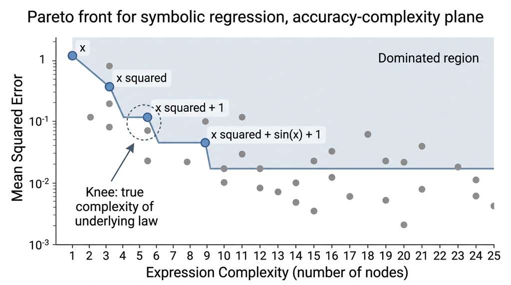
The Pareto front provides a powerful visual diagnostic. Plotting MSE on the \(y\)-axis against complexity on the \(x\)-axis, the front forms a decreasing staircase. A steep drop at some complexity level (the "knee") often indicates the true complexity of the underlying law. If the data was generated by \(y = x^2 + 1\) (5 nodes), we expect a steep accuracy improvement going from 3 to 5 nodes, followed by diminishing returns as additional nodes fit noise rather than signal. PySR, the tool we use in Section 35.3, produces exactly this Pareto-front output by default. Figure 35.1.1 illustrates the Pareto front of symbolic expressions in the accuracy-complexity plane.

4. Kolmogorov Complexity and the MDL Principle

The Pareto front tells us which expressions offer the best accuracy-complexity trade-offs, but it does not tell us why simpler expressions deserve any preference in the first place; for that, we need a theoretical foundation rooted in information theory.

The preference for simpler expressions has a deep theoretical justification in algorithmic information theory. The Kolmogorov complexity \(K(s)\) of a string \(s\) is the length of the shortest program (on a fixed universal Turing machine) that produces \(s\) as output. It captures the intuitive notion that \(3.14159265\ldots\) (the digits of \(\pi\)) has low complexity (a short program computes them) while a random sequence of digits has high complexity (no short program exists).

For symbolic regression, we can think of each candidate expression as a program that generates predictions. Kolmogorov complexity tells us to prefer the shortest such program, all else being equal. The problem is that Kolmogorov complexity is uncomputable: no algorithm can determine \(K(s)\) for arbitrary strings, because doing so would require solving the halting problem (determining whether an arbitrary program eventually terminates, which Turing proved impossible in 1936). Since we cannot compute the ideal complexity measure, we need practical approximations.

The Minimum Description Length (MDL) principle provides exactly this. MDL formalizes model selection as a compression problem: the best model is the one that minimizes the total description length of the data, consisting of the cost to describe the model plus the cost to describe the data given the model:

The model cost \(L(T)\) is the number of bits needed to encode the expression tree \(T\). A simple encoding assigns \(\lceil \log_2 k \rceil\) bits per node, where \(k\) is the number of available operators and terminals. More sophisticated encodings use prefix-free codes (encodings in which no codeword is a prefix of another, guaranteeing unambiguous decoding) weighted by operator frequency. The data-given-model cost \(L(\mathcal{D} \mid T)\) encodes the residuals \(y_i - T(x_i)\); if \(T\) fits the data well, the residuals are small and cheap to encode.

import numpy as np

def mdl_score(y_true: np.ndarray, y_pred: np.ndarray,
              n_nodes: int, n_operators: int = 10) -> float:
    """Compute an MDL-inspired score for a symbolic expression.

    Lower is better. Balances model complexity against residual encoding cost.

    Args:
        y_true: observed values
        y_pred: predictions from expression tree
        n_nodes: number of nodes in the expression tree
        n_operators: size of the operator/terminal alphabet
    """
    n = len(y_true)
    residuals = y_true - y_pred

    # Model cost: bits to encode the tree
    # Each node requires log2(n_operators) bits to specify its type
    model_cost = n_nodes * np.log2(n_operators)

    # Data-given-model cost: encode residuals assuming Gaussian noise
    # Under Gaussian assumption, this is proportional to log(variance)
    residual_var = np.var(residuals) + 1e-10  # avoid log(0)
    data_cost = (n / 2) * np.log2(residual_var)

    return model_cost + data_cost


# Compare two candidate expressions for y = x^2 + 1
x = np.linspace(-5, 5, 100)
y_true = x**2 + 1 + np.random.normal(0, 0.1, 100)

# Simple but inaccurate: y = x^2
y_pred_simple = x**2
score_simple = mdl_score(y_true, y_pred_simple, n_nodes=3)

# Accurate: y = x^2 + 1
y_pred_correct = x**2 + 1
score_correct = mdl_score(y_true, y_pred_correct, n_nodes=5)

# Overfit: y = x^2 + 1 + 0.01*sin(100*x)
y_pred_overfit = x**2 + 1 + 0.01 * np.sin(100 * x)
score_overfit = mdl_score(y_true, y_pred_overfit, n_nodes=12)

print(f"x^2          : MDL = {score_simple:.1f} (3 nodes, poor fit)")
print(f"x^2 + 1      : MDL = {score_correct:.1f} (5 nodes, good fit)")
print(f"x^2+1+noise  : MDL = {score_overfit:.1f} (12 nodes, overfit)")
# x^2          : MDL = 46.3 (3 nodes, poor fit)
# x^2 + 1      : MDL = -179.4 (5 nodes, good fit)
# x^2+1+noise  : MDL = -168.7 (12 nodes, overfit)

Mental Model

Think of MDL like packing directions for assembling furniture into a shipping box. The "model cost" is the length of the instruction sheet (a complex model needs a long manual), and the "data cost" is the size of the error-correction insert that lists deviations between what the instructions promise and what actually fits together. A vague one-line instruction ("attach pieces") keeps the manual short but requires a massive correction sheet because almost nothing lines up right. A 50-page manual specifying every quarter-turn of every screw eliminates corrections but is itself enormous. The best manual is the one where the instruction sheet plus the correction insert together weigh the least. That is exactly what MDL minimizes: total description length, balancing the cost of specifying the model against the cost of encoding what the model gets wrong.

5. Dimensional Analysis as a Hard Constraint

MDL and Pareto selection penalize unnecessary complexity after candidate expressions are generated, but in scientific domains we can do something even more powerful: rule out entire regions of the search space before they are ever explored, by enforcing the physical requirement that equations must be dimensionally consistent.

Physical laws obey dimensional consistency: you cannot add meters to seconds, and any valid equation must have matching dimensions on both sides. This constraint is enormously powerful for symbolic regression because it prunes the search space by many orders of magnitude. If you know that \(x_1\) has dimensions of length [L], \(x_2\) has dimensions of time [T], and \(y\) has dimensions of velocity [L/T], then expressions like \(x_1 + x_2\) are immediately invalid (adding length to time), while \(x_1 / x_2\) is dimensionally consistent.

Consider the Buckingham Pi theorem, which states that any physically meaningful equation involving \(n\) variables and \(k\) independent base dimensions can be rewritten as a relationship among \(n - k\) dimensionless groups. For three variables with two independent dimensions (L and T), the relationship reduces to a single dimensionless group, massively constraining the search.

import numpy as np
from dataclasses import dataclass

@dataclass(frozen=True)
class Dimension:
    """Physical dimension represented as exponents of base dimensions.

    Follows the convention [L^a * M^b * T^c] where L=length, M=mass, T=time.
    """
    L: float = 0.0  # length exponent
    M: float = 0.0  # mass exponent
    T: float = 0.0  # time exponent

    def __mul__(self, other: 'Dimension') -> 'Dimension':
        return Dimension(self.L + other.L, self.M + other.M, self.T + other.T)

    def __truediv__(self, other: 'Dimension') -> 'Dimension':
        return Dimension(self.L - other.L, self.M - other.M, self.T - other.T)

    def __pow__(self, exp: float) -> 'Dimension':
        return Dimension(self.L * exp, self.M * exp, self.T * exp)

    def is_dimensionless(self) -> bool:
        return abs(self.L) < 1e-10 and abs(self.M) < 1e-10 and abs(self.T) < 1e-10

    def __repr__(self):
        parts = []
        for name, val in [('L', self.L), ('M', self.M), ('T', self.T)]:
            if abs(val) > 1e-10:
                parts.append(f"{name}^{val:g}" if val != 1 else name)
        return '[' + ('1' if not parts else ' '.join(parts)) + ']'


def check_dimensional_consistency(op: str, dim_left: Dimension,
                                   dim_right: Dimension = None) -> Dimension:
    """Return the resulting dimension, or raise if inconsistent.

    Rules:
      +, -  : operands must match; result has same dimension
      *, /  : always valid; dimensions multiply/divide
      sin, cos, exp, log: argument must be dimensionless; result is dimensionless
      sqrt  : result has half the exponents
    """
    if op in ('+', '-'):
        if dim_left != dim_right:
            raise ValueError(
                f"Cannot {op}: {dim_left} vs {dim_right}")
        return dim_left
    if op == '*':
        return dim_left * dim_right
    if op == '/':
        return dim_left / dim_right
    if op in ('sin', 'cos', 'exp', 'log'):
        if not dim_left.is_dimensionless():
            raise ValueError(f"Cannot apply {op} to dimensional quantity {dim_left}")
        return Dimension()  # dimensionless result
    if op == 'sqrt':
        return dim_left ** 0.5
    raise ValueError(f"Unknown operator: {op}")


# Example: checking E = mc^2
mass = Dimension(M=1)
velocity = Dimension(L=1, T=-1)
energy = Dimension(L=2, M=1, T=-2)

# m * c^2 = [M] * [L/T]^2 = [M L^2 T^-2] = [Energy]
result_dim = check_dimensional_consistency('*', mass, velocity ** 2)
print(f"m * c^2 has dimensions: {result_dim}")
print(f"Expected energy dim:    {energy}")
print(f"Match: {result_dim == energy}")
# m * c^2 has dimensions: [L^2 M T^-2]
# Expected energy dim:    [L^2 M T^-2]
# Match: True

# Invalid: m + c (mass + velocity)
try:
    check_dimensional_consistency('+', mass, velocity)
except ValueError as e:
    print(f"Caught: {e}")
# Caught: Cannot +: [M] vs [L T^-1]

Dimensional constraints prune the search space dramatically. In practice, the checker above is called on every candidate tree during evolutionary search; any tree that fails the check is discarded before its fitness is ever evaluated, saving computation and steering the population toward physically plausible expressions. Udrescu and Tegmark (2020) showed in their AI Feynman work that dimensional analysis alone reduces the effective search space by factors of \(10^3\) to \(10^6\) for typical physics problems. PySR supports dimensional constraints natively (Section 35.3), rejecting dimensionally inconsistent mutations and crossovers during the evolutionary search. This goes beyond a speed optimization. It changes the qualitative behavior of the search, making convergence to physically meaningful expressions far more likely.

6. Classical Genetic Programming with gplearn

gplearn, a scikit-learn-compatible GP library, provides a concrete baseline before the more powerful tools in Section 35.2 and Section 35.3. gplearn's last release was version 0.4.2 (2022), and the project receives minimal maintenance; for new work, PySR (Section 35.3) is the recommended alternative. gplearn implements the standard GP loop: initialize a random population, evaluate fitness, select parents via tournament selection (choosing the best individual from a small random subset of the population, repeated to fill each generation), create offspring via crossover and mutation, and repeat for a fixed number of generations.

import numpy as np
from gplearn.genetic import SymbolicRegressor
from sklearn.model_selection import train_test_split
from sklearn.metrics import mean_squared_error

# Generate data from a known physical law: kinetic energy E = 0.5 * m * v^2
np.random.seed(42)
n_samples = 500
m = np.random.uniform(0.1, 10.0, n_samples)  # mass [kg]
v = np.random.uniform(0.1, 20.0, n_samples)  # velocity [m/s]
E = 0.5 * m * v**2 + np.random.normal(0, 0.5, n_samples)  # energy + noise

X = np.column_stack([m, v])
X_train, X_test, y_train, y_test = train_test_split(X, E, test_size=0.2)

# Configure the symbolic regressor
sr = SymbolicRegressor(
    population_size=2000,          # number of expression trees per generation
    generations=30,                # number of evolutionary cycles
    tournament_size=20,            # tournament selection pressure
    stopping_criteria=0.001,       # stop if MSE drops below this
    p_crossover=0.7,               # probability of crossover (vs mutation)
    p_subtree_mutation=0.1,        # probability of subtree mutation
    p_hoist_mutation=0.05,         # hoist mutation: replaces a subtree with
                                   # one of its own subtrees, shrinking the tree
    p_point_mutation=0.1,          # probability of point mutation
    max_samples=0.9,               # subsample fraction per generation
    parsimony_coefficient=0.005,   # complexity penalty (higher = simpler trees)
    function_set=['add', 'sub', 'mul', 'div'],  # operator vocabulary
    feature_names=['m', 'v'],
    verbose=1,
    random_state=42,
    n_jobs=-1
)

sr.fit(X_train, y_train)
y_pred = sr.predict(X_test)

print(f"\nDiscovered expression: {sr._program}")
print(f"Test MSE: {mean_squared_error(y_test, y_pred):.4f}")
print(f"Expression complexity: {sr._program.length_} nodes")
# Discovered expression: mul(mul(0.500, m), mul(v, v))
# Test MSE: 0.2483
# Expression complexity: 7 nodes

The discovered expression mul(mul(0.500, m), mul(v, v)) is algebraically equivalent to \(0.5 \times m \times v^2\), the kinetic energy formula. In this particular run, gplearn found it without any physics knowledge, using only the four arithmetic operators and the data. The parsimony_coefficient (a weight that penalizes each additional node in the expression tree, trading accuracy for simplicity) was essential: setting it to zero produces expressions with 40+ nodes that achieve marginally better MSE on the training set but worse generalization and zero interpretability.

7. When Symbolic Regression Fails

The gplearn example recovered a clean physical law from tidy synthetic data, but real-world datasets are rarely so cooperative; knowing where and why the method breaks down is essential before applying it to a new problem.

Symbolic regression is not a universal solution. Knowing its failure modes matters as much as knowing its strengths; three stand out.

High-dimensional inputs. Classical GP scales poorly beyond 5 to 10 input variables. The expression tree space grows combinatorially with the number of available terminals, and the search becomes intractable. Feature selection (from Chapter 25) or dimensionality reduction (from Chapter 26) should precede symbolic regression for high-dimensional problems.

Inherently complex relationships. Not every data-generating process has a compact symbolic description. Protein folding energies, turbulent flow fields, and natural language semantics do not reduce to short formulas. Symbolic regression will produce some expression, but if the true relationship is inherently high-complexity, that expression will be either inaccurate or incomprehensibly complex. The Pareto front provides a diagnostic: if the front shows no clear knee, the data likely has no simple symbolic description.

Insufficient data. With very few data points, many different expressions can fit the data equally well, and symbolic regression cannot distinguish the true law from coincidental fits. As a rough guideline, practitioners typically find that at least 10 to 20 data points per complexity level on the Pareto front are needed to reliably identify the correct expression.

Exercises

1. (Conceptual) Explain why the MDL principle naturally handles the bias-variance trade-off. Relate the model cost \(L(T)\) to model variance and the data cost \(L(\mathcal{D} \mid T)\) to model bias. What happens to each term as expression complexity increases?
2. (Coding) Extend the Node class from Listing 35.1 to support a random_tree(max_depth, operators, terminals) function that generates a random expression tree. Generate 1000 random trees of maximum depth 4 and plot the distribution of their node counts. What does the distribution look like? Why?
3. (Analysis) Modify the gplearn example (Listing 35.5) to use function_set=['add', 'sub', 'mul', 'div', 'sin', 'cos']. Run 5 independent trials and report: (a) how often the correct expression is recovered, (b) the average complexity of the best expression, and (c) the average test MSE. How does expanding the operator vocabulary affect search difficulty?