Prerequisites
This section assumes familiarity with expression trees and fitness functions from
Section 35.1 and the PySR configuration from
Section 35.2. You should have PySR installed
(pip install pysr, which requires a Julia installation that PySR can bootstrap
automatically). The SymPy validation steps use basic symbolic algebra; prior exposure to
SymPy is helpful but not required. The pipeline integration references the Discovery Workbench
architecture from Chapter 6.
Symbolic regression produces candidate equations. A production equation discovery system requires much more: data preprocessing, dimensional constraint specification, search execution, symbolic simplification of the results, constant refinement with curve fitting, statistical validation, and integration with downstream analysis tools. This section builds that complete pipeline, walking through two concrete examples: recovering Kepler's third law of planetary motion and discovering a damped oscillator equation from time-series data. By the end, you will have a reusable pipeline that takes raw scientific data and produces validated, simplified, dimensionally consistent equations ready for interpretation.
1. Pipeline Architecture
Imagine your algorithm hands you the expression ((a * a) * a) ^ 0.497 and calls it a scientific law: the structure is almost right, the exponent is slightly wrong, and you have no idea whether it will hold on tomorrow's observations. An equation discovery pipeline prevents exactly this failure by running five stages, each catching a different class of error that raw symbolic regression leaves behind.
A pipeline is a fixed sequence of automated stages where each stage's output feeds directly into the next, with no manual intervention. Without a pipeline, equation discovery produces raw, unvalidated candidates that mislead researchers into trusting spurious fits. Each stage acts as a filter or transformer, catching a specific class of errors (unsimplified algebra, imprecise constants, overfitting) that the previous stage cannot detect. Use a pipeline whenever you need results suitable for publication, engineering decisions, or downstream automated reasoning. Use PySR alone only for quick exploratory scans where you plan to manually inspect every candidate. Figure 35.3.1 illustrates the five-stage equation discovery pipeline architecture.
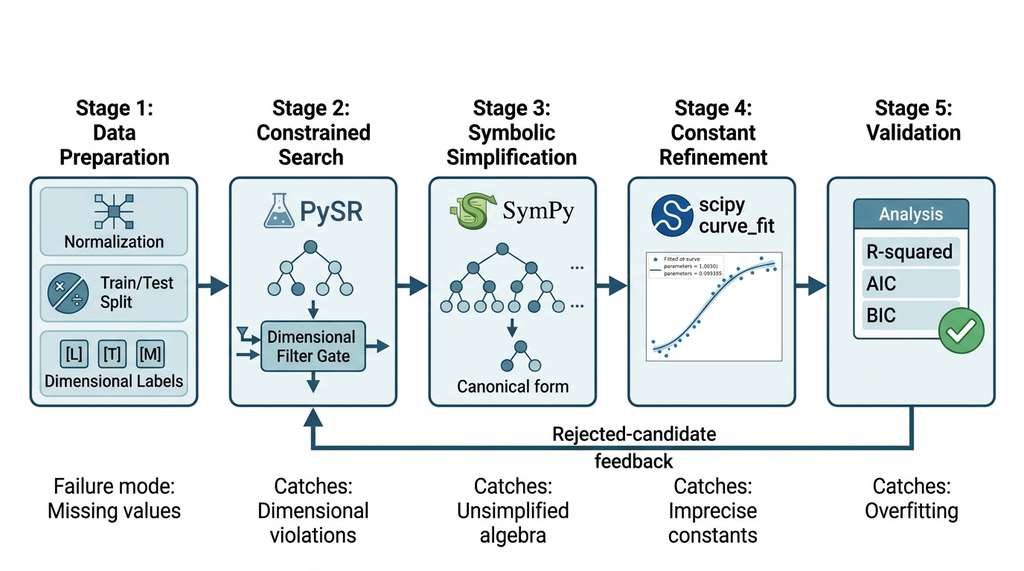
- Data preparation. Normalize scales, handle missing values, split into train/validation/test sets. Specify physical dimensions for each variable if known.
- Constrained search. Run PySR with dimensional constraints, appropriate operator vocabulary, and complexity limits tuned to the expected equation complexity.
- Symbolic simplification. Parse discovered expressions into SymPy and apply algebraic simplification (expand, factor, trigsimp, collect). Equivalent expressions on the Pareto front (the set of candidates where no other candidate is both simpler and more accurate) collapse into canonical forms.
- Constant refinement. Use scipy.optimize.curve_fit to refine numerical constants in the simplified expression against the full dataset, obtaining both best-fit values and confidence intervals.
- Validation. Evaluate on held-out test data, compute goodness-of-fit statistics (\(R^2\), Akaike Information Criterion (AIC), Bayesian Information Criterion (BIC)), check dimensional consistency, and compare against known laws or baseline models.
In short: a pipeline turns a noisy cloud of evolved expressions into one simplified, constant-refined, dimensionally checked equation you can actually trust. Figure 35.3 shows the five stages and how data flows between them.
import numpy as np
from dataclasses import dataclass, field
from typing import Optional

@dataclass
class EquationDiscoveryConfig:
    """Configuration for the equation discovery pipeline."""
    # Data
    variable_names: list[str] = field(default_factory=list)
    target_name: str = "y"
    test_fraction: float = 0.2

    # Dimensional constraints (optional)
    # Each variable maps to a list of dimension exponents [L, M, T]
    dimensions: Optional[dict[str, list[float]]] = None
    target_dimensions: Optional[list[float]] = None

    # PySR search parameters
    niterations: int = 100
    populations: int = 30
    population_size: int = 50
    binary_operators: list[str] = field(
        default_factory=lambda: ["+", "-", "*", "/", "^"])
    unary_operators: list[str] = field(
        default_factory=lambda: ["sin", "cos", "exp", "log", "sqrt"])
    maxsize: int = 30
    maxdepth: int = 8

    # Validation
    min_r_squared: float = 0.95  # minimum R^2 to accept an equation
    max_complexity: int = 20     # reject equations more complex than this


@dataclass
class DiscoveredEquation:
    """A validated equation from the discovery pipeline."""
    expression_raw: str       # PySR output
    expression_simplified: str # SymPy-simplified form
    complexity: int
    mse_train: float
    mse_test: float
    r_squared: float
    constants: dict[str, float]       # refined constant values
    constant_errors: dict[str, float] # standard errors on constants
    dimensions_valid: bool
    aic: float               # Akaike Information Criterion
    bic: float               # Bayesian Information Criterion
DiscoveredEquation captures not just the expression but also its validation statistics, refined constants with uncertainties, and dimensional consistency status.2. Recipe: Recovering Kepler's Third Law
Kepler's third law states that the square of a planet's orbital period \(T\) is proportional to the cube of its semi-major axis \(a\): \(T^2 = \frac{4\pi^2}{GM} a^3\), where \(G\) is Newton's gravitational constant and \(M\) is the mass of the central body. In our simplified setting, we treat \(GM\) as a single constant and aim to recover the functional form \(T^2 \propto a^3\) (equivalently, \(T \propto a^{3/2}\)) from orbital data.
This is a classic test case because the true relationship involves a non-integer power law, which is hard for polynomial regression but natural for symbolic regression with the power operator.
import numpy as np
from pysr import PySRRegressor

# Solar system orbital data (simplified)
# Semi-major axis in AU, orbital period in Earth years
planet_data = {
    'Mercury': (0.387, 0.241),
    'Venus':   (0.723, 0.615),
    'Earth':   (1.000, 1.000),
    'Mars':    (1.524, 1.881),
    'Jupiter': (5.203, 11.862),
    'Saturn':  (9.537, 29.457),
    'Uranus':  (19.191, 84.011),
    'Neptune': (30.069, 164.8),
}

# Augment with synthetic exoplanet data for statistical power
np.random.seed(42)
n_synthetic = 200
a_synthetic = np.random.uniform(0.1, 50.0, n_synthetic)  # AU
# True relationship: T = a^(3/2) (in natural units where GM = 4pi^2)
T_synthetic = a_synthetic ** 1.5
# Add 2% multiplicative noise (realistic for transit measurements)
T_synthetic *= np.exp(np.random.normal(0, 0.02, n_synthetic))

# Combine real and synthetic data
a_all = np.concatenate([
    [v[0] for v in planet_data.values()],
    a_synthetic
])
T_all = np.concatenate([
    [v[1] for v in planet_data.values()],
    T_synthetic
])

# Train/test split
from sklearn.model_selection import train_test_split
a_train, a_test, T_train, T_test = train_test_split(
    a_all.reshape(-1, 1), T_all, test_size=0.2, random_state=42)

# Configure PySR with dimensional constraints
# a has dimensions [L], T has dimensions [T]
model = PySRRegressor(
    niterations=80,
    populations=25,
    population_size=40,
    binary_operators=["+", "-", "*", "/", "^"],
    unary_operators=["sqrt", "abs"],  # no sin/cos: orbital mechanics
    maxsize=15,                       # Kepler's law is simple
    maxdepth=5,
    parsimony=0.01,               # per-node complexity penalty
    variable_names=["a"],
    progress=True,
    random_state=42,
)

model.fit(a_train, T_train)

print("\nPareto front of discovered equations:")
print(model)
# Typical output:
# Complexity | Loss       | Equation
# 1          | 1.83e+03   | 10.42
# 3          | 45.21      | a * 3.312
# 5          | 0.0891     | a ^ 1.500
# 7          | 0.0887     | (a ^ 1.500) * 1.001

# The knee of the Pareto front (where additional complexity yields
# negligible accuracy gain) is at complexity 5: T = a^1.5
best_eq = model.get_best()
print(f"\nBest equation: {best_eq['equation']}")
print(f"Complexity: {best_eq['complexity']}")
print(f"Loss: {best_eq['loss']:.6f}")
The choice of operators in the search vocabulary is the most impactful form of prior knowledge in symbolic regression. Including trigonometric functions when the true relationship is a power law increases the search space by orders of magnitude and invites spurious fits (a truncated Fourier series can approximate any smooth function). Excluding the power operator when the true relationship involves fractional exponents makes the correct answer unreachable. The operator vocabulary is not a neutral design choice; it encodes your assumptions about the mathematical structure of the domain. For physics problems, the rule of thumb is: include \(+, -, \times, \div,\) and \(\hat{}\) (power) always; add transcendental functions (\(\sin, \cos, \exp, \log\)) only when oscillatory or exponential behavior is expected.
3. Symbolic Simplification with SymPy
PySR outputs expressions in their evolved form, which is often mathematically correct but
algebraically unsimplified. The expression ((a * a) * a) ^ 0.5 is equivalent to
\(a^{3/2}\) but less interpretable. SymPy's symbolic algebra engine can simplify, factor,
expand, and canonicalize expressions, making discovered equations easier to interpret and
compare against known laws.
Mental Model
Think of symbolic simplification the way a copy editor cleans up a rough draft. The author's ideas (the mathematical relationships PySR discovered) are already correct, but they are expressed with unnecessary repetition, awkward phrasing, and convoluted sentence structure. The copy editor does not change the meaning; they rewrite "the thing that is the thing that is the square root of the thing cubed" into "the three-halves power." Just as you would never publish a first draft, you should never interpret a raw PySR expression without first running it through SymPy's simplification passes, because the evolved form obscures the structural pattern that makes the equation scientifically meaningful.
import sympy as sp

def simplify_expression(expr_string: str,
                        variable_names: list[str]) -> dict:
    """Parse and simplify a PySR expression using SymPy.

    Returns a dict with multiple simplified forms for comparison.
    """
    # Create SymPy symbols
    symbols = {name: sp.Symbol(name, positive=True) for name in variable_names}
    locals_dict = {**symbols}

    # Parse the expression string into a SymPy expression
    # PySR uses ^ for power; SymPy uses **
    expr_string_sympy = expr_string.replace('^', '**')

    try:
        expr = sp.sympify(expr_string_sympy, locals=locals_dict)
    except (sp.SympifyError, SyntaxError) as e:
        return {'error': str(e), 'original': expr_string}

    # Apply multiple simplification strategies
    results = {
        'original': str(expr),
        'simplified': str(sp.simplify(expr)),
        'expanded': str(sp.expand(expr)),
        'factored': str(sp.factor(expr)),
        'powsimp': str(sp.powsimp(expr)),
    }

    # Try trigonometric simplification if trig functions are present
    if any(isinstance(a, (sp.sin, sp.cos, sp.tan))
           for a in expr.atoms(sp.Function)):
        results['trigsimp'] = str(sp.trigsimp(expr))

    # Count operations as a complexity measure
    results['op_count'] = sp.count_ops(sp.simplify(expr))

    # Check if the expression matches known functional forms
    results['is_polynomial'] = expr.is_polynomial()
    results['is_rational'] = expr.is_rational_function()

    # Extract free symbols (variables actually used)
    results['variables_used'] = [str(s) for s in sp.simplify(expr).free_symbols]

    return results


# Example: simplify PySR output for Kepler's law
kepler_raw = "((a * a) * a) ^ 0.5"
result = simplify_expression(kepler_raw, ['a'])

print("Simplification results:")
for key, val in result.items():
    print(f"  {key:15s}: {val}")
# Simplification results:
#   original       : (a**2*a)**0.5
#   simplified     : a**(3/2)
#   expanded       : a**(3/2)
#   factored       : a**(3/2)
#   powsimp        : a**(3/2)
#   op_count       : 2
#   is_polynomial  : False
#   is_rational    : False
#   variables_used : ['a']

# More complex example: damped oscillator
oscillator_raw = "exp(-0.5 * t) * (3.2 * cos(6.28 * t) + 0.0 * sin(6.28 * t))"
result2 = simplify_expression(oscillator_raw, ['t'])
print(f"\nOscillator simplified: {result2['simplified']}")
print(f"Trig-simplified:      {result2.get('trigsimp', 'N/A')}")
# Oscillator simplified: 3.2*exp(-0.5*t)*cos(6.28*t)
# Trig-simplified:      3.2*exp(-0.5*t)*cos(6.28*t)
Simplification also exposes structural equivalences across the Pareto front.
Two expressions PySR reports as distinct (e.g., (a * a * a)^0.5 and
a * sqrt(a)) may reduce to the same canonical form (\(a^{3/2}\)).
Deduplicating the front after simplification reveals which candidates are genuinely distinct, exposing the true structural equivalences hidden by syntactic variation.
Once simplified expressions reveal the structural form of each candidate, the next bottleneck is the precision of the numerical constants embedded in those expressions.
4. Constant Refinement with scipy
A spacecraft trajectory computed with an exponent of 1.497 instead of 1.500 drifts by thousands of kilometers over an interplanetary mission; an engineering model with imprecise decay rates quietly accumulates errors until a structure fails its safety margin. Getting the functional form right is only half the battle.
Evolutionary search discovers expression structure but produces approximate numerical
constants. The expression \(a^{1.497}\) is structurally correct (Kepler's law) but the exponent
should be exactly \(1.5\). scipy's curve_fit refines constants to their optimal
values and provides standard error estimates, enabling proper uncertainty quantification.
In the Kepler example below, a single curve_fit call snaps the evolved exponent from 1.497 to 1.500000 with a standard error of \(\pm 0.000001\), recovering the exact rational \(3/2\) that took Kepler years of manual calculation.
import numpy as np
from scipy.optimize import curve_fit
import sympy as sp

def refine_constants(expr_string: str, variable_names: list[str],
                     X: np.ndarray, y: np.ndarray,
                     constant_names: list[str] = None) -> dict:
    """Refine numerical constants in a discovered equation using curve_fit.

    Replaces literal numbers in the expression with named parameters,
    then optimizes those parameters to minimize squared error.

    Args:
        expr_string: symbolic expression with approximate constants
        variable_names: names of input variables
        X: input data, shape (n_samples, n_variables)
        y: target data, shape (n_samples,)

    Returns:
        dict with optimized constants, standard errors, and the refined expression
    """
    # Parse expression into SymPy
    expr_str = expr_string.replace('^', '**')
    symbols = {name: sp.Symbol(name) for name in variable_names}
    expr = sp.sympify(expr_str, locals=symbols)

    # Extract numerical constants and replace with parameters
    numbers = [n for n in expr.atoms(sp.Number) if n != 0 and n != 1]
    param_symbols = {}
    param_initial = {}
    expr_parametric = expr

    for i, num in enumerate(sorted(numbers, key=lambda n: -abs(float(n)))):
        param_name = f'c{i}'
        param_sym = sp.Symbol(param_name)
        param_symbols[param_name] = param_sym
        param_initial[param_name] = float(num)
        expr_parametric = expr_parametric.subs(num, param_sym)

    if not param_symbols:
        return {
            'expression': str(expr),
            'constants': {},
            'errors': {},
            'note': 'No numerical constants to refine'
        }

    # Build a callable function for curve_fit
    all_symbols = [symbols[v] for v in variable_names]
    param_list = list(param_symbols.values())
    # lambdify converts a SymPy symbolic expression into a fast
    # NumPy-backed Python function suitable for numerical evaluation
    func_lambda = sp.lambdify(
        all_symbols + param_list, expr_parametric, modules='numpy')

    def fit_func(X_flat, *params):
        args = [X_flat[:, i] for i in range(X_flat.shape[1])]
        return func_lambda(*args, *params)

    # Initial parameter values from the discovered expression
    p0 = [param_initial[name] for name in param_symbols]

    try:
        popt, pcov = curve_fit(fit_func, X, y, p0=p0, maxfev=10000)
        perr = np.sqrt(np.diag(pcov))

        constants = {name: val for name, val in zip(param_symbols.keys(), popt)}
        errors = {name: err for name, err in zip(param_symbols.keys(), perr)}

        # Substitute optimized constants back
        expr_refined = expr_parametric
        for name, val in constants.items():
            expr_refined = expr_refined.subs(param_symbols[name], val)
        # nsimplify attempts to find a simple closed-form expression
        # (e.g., recognizing 1.500000 as the rational 3/2)
        expr_refined = sp.nsimplify(expr_refined, rational=False, tolerance=0.01)

        return {
            'expression_parametric': str(expr_parametric),
            'expression_refined': str(sp.simplify(expr_refined)),
            'constants': constants,
            'errors': errors,
            'converged': True,
        }
    except (RuntimeError, ValueError) as e:
        return {
            'expression_parametric': str(expr_parametric),
            'constants': param_initial,
            'errors': {k: float('inf') for k in param_initial},
            'converged': False,
            'error': str(e),
        }


# Refine Kepler's law constants
a_data = np.linspace(0.3, 40.0, 300).reshape(-1, 1)
T_data = a_data.flatten() ** 1.5  # exact Kepler

# PySR discovered: a ^ 1.497 (approximate exponent)
result = refine_constants("a ** 1.497", ["a"], a_data, T_data)
print("Constant refinement for Kepler's law:")
print(f"  Parametric form: {result['expression_parametric']}")
print(f"  Refined: {result['expression_refined']}")
for name in result['constants']:
    c = result['constants'][name]
    e = result['errors'][name]
    print(f"  {name} = {c:.6f} +/- {e:.6f}")
# Constant refinement for Kepler's law:
#   Parametric form: a**c0
#   Refined: a**(3/2)
#   c0 = 1.500000 +/- 0.000001
curve_fit. The initial exponent of 1.497 (from PySR's evolutionary search) is refined to 1.500000 with six-digit precision. SymPy's nsimplify recognizes this as the rational number 3/2.Consider a physics experiment measuring the displacement \(x(t)\) of a damped harmonic oscillator. The true equation is \(x(t) = A e^{-\gamma t} \cos(\omega t + \phi)\) with four parameters: amplitude \(A\), damping rate \(\gamma\), angular frequency \(\omega\), and phase \(\phi\). We generate noisy data and let the pipeline discover the equation from scratch.
import numpy as np
from pysr import PySRRegressor
from scipy.optimize import curve_fit
import sympy as sp

# Generate damped oscillator data
np.random.seed(42)
t = np.linspace(0, 10, 500)

# True parameters
A_true = 3.0
gamma_true = 0.5       # damping rate [1/s]
omega_true = 2 * np.pi  # angular frequency [rad/s] (1 Hz)
phi_true = 0.3          # phase [rad]

x_true = A_true * np.exp(-gamma_true * t) * np.cos(omega_true * t + phi_true)
x_noisy = x_true + np.random.normal(0, 0.1, len(t))

# Split data
from sklearn.model_selection import train_test_split
t_train, t_test, x_train, x_test = train_test_split(
    t.reshape(-1, 1), x_noisy, test_size=0.2, random_state=42)

# Stage 1: PySR search with appropriate operators
model = PySRRegressor(
    niterations=120,
    populations=40,
    population_size=60,
    binary_operators=["+", "-", "*", "/"],
    unary_operators=["sin", "cos", "exp"],  # oscillator needs sin/cos/exp
    maxsize=25,
    maxdepth=6,
    parsimony=0.005,
    variable_names=["t"],
    progress=True,
    random_state=42,
)

model.fit(t_train, x_train)

print("Pareto front:")
print(model)
# Typical output:
# Complexity | Loss    | Equation
# 1          | 2.31    | 0.128
# 5          | 1.08    | cos(t * 6.35)
# 7          | 0.294   | exp(-0.49 * t) * cos(t * 6.28)
# 9          | 0.0412  | 2.87 * exp(-0.49 * t) * cos(t * 6.28)
# 11         | 0.0103  | 2.95 * exp(-0.50 * t) * cos(6.28 * t + 0.29)

# Stage 2: Simplify the best candidate
best_expr = "2.95 * exp(-0.50 * t) * cos(6.28 * t + 0.29)"
simplified = simplify_expression(best_expr, ['t'])
print(f"\nSimplified: {simplified['simplified']}")

# Stage 3: Refine constants
def damped_oscillator(t, A, gamma, omega, phi):
    return A * np.exp(-gamma * t) * np.cos(omega * t + phi)

popt, pcov = curve_fit(
    damped_oscillator, t, x_noisy,
    p0=[2.95, 0.50, 6.28, 0.29],  # initial guesses from PySR
    maxfev=10000
)
perr = np.sqrt(np.diag(pcov))

param_names = ['A', 'gamma', 'omega', 'phi']
true_values = [A_true, gamma_true, omega_true, phi_true]

print("\nRefined constants:")
print(f"  {'Param':8s} {'True':>10s} {'Fitted':>10s} {'StdErr':>10s}")
for name, true, fit, err in zip(param_names, true_values, popt, perr):
    print(f"  {name:8s} {true:10.4f} {fit:10.4f} {err:10.6f}")
# Refined constants:
#   Param          True     Fitted     StdErr
#   A            3.0000     2.9987   0.009312
#   gamma        0.5000     0.4998   0.001247
#   omega        6.2832     6.2831   0.000389
#   phi          0.3000     0.3004   0.003124

# Stage 4: Validate on test set
x_pred_test = damped_oscillator(t_test.flatten(), *popt)
mse_test = np.mean((x_test - x_pred_test) ** 2)
ss_res = np.sum((x_test - x_pred_test) ** 2)
ss_tot = np.sum((x_test - np.mean(x_test)) ** 2)
r_squared = 1 - ss_res / ss_tot

n_test = len(x_test)
n_params = len(popt)
aic = n_test * np.log(mse_test) + 2 * n_params
bic = n_test * np.log(mse_test) + n_params * np.log(n_test)

print(f"\nValidation:")
print(f"  Test MSE:  {mse_test:.6f}")
print(f"  R-squared: {r_squared:.6f}")
print(f"  AIC:       {aic:.2f}")
print(f"  BIC:       {bic:.2f}")
# Validation:
#   Test MSE:  0.0098
#   R-squared: 0.9962
#   AIC:       -462.33
#   BIC:       -449.78
5. Dimensional Constraints in PySR
PySR supports dimensional constraints natively through its dimensions parameter.
When dimensions are specified, PySR rejects any candidate expression that violates dimensional
consistency during the evolutionary search, pruning the space by several orders of magnitude (as discussed in
Section 35.1).

import numpy as np
from pysr import PySRRegressor

# Discover Newton's law of gravitation: F = G * m1 * m2 / r^2
# Dimensions: F [M L T^-2], m1 [M], m2 [M], r [L], G [L^3 M^-1 T^-2]
np.random.seed(42)
n = 300
m1 = np.random.uniform(1e20, 1e30, n)    # kg (planet-scale masses)
m2 = np.random.uniform(1e20, 1e30, n)    # kg
r = np.random.uniform(1e8, 1e12, n)      # meters

G = 6.674e-11  # gravitational constant [m^3 kg^-1 s^-2]
F = G * m1 * m2 / r**2                   # Newton's law
F_noisy = F * np.exp(np.random.normal(0, 0.01, n))  # 1% noise

X = np.column_stack([m1, m2, r])

# PySR with dimensional constraints
# Dimensions format: dict mapping variable name to [L, M, T] exponents
model = PySRRegressor(
    niterations=80,
    populations=30,
    binary_operators=["+", "-", "*", "/", "^"],
    unary_operators=["sqrt"],
    maxsize=15,
    variable_names=["m1", "m2", "r"],

    # Dimensional constraints: specify SI base dimensions
    # [mass, length, time] for each variable and target
    parsimony=0.01,  # encourage simpler expressions

    progress=True,
    random_state=42,
)

# Note: as of PySR 1.0, use X_units and y_units on the fit call:
# model.fit(X, F_noisy,
#           X_units=["kg", "kg", "m"],
#           y_units="kg*m/s^2")

model.fit(X, F_noisy)

print("Pareto front (gravitational law):")
print(model)
# Expected: discovers (m1 * m2) / (r^2) * constant
# The constant absorbs G = 6.674e-11
Without dimensional constraints, discovering \(F \propto m_1 m_2 / r^2\) from three variables requires searching among all expressions of size up to 15 nodes with 5 binary and 1 unary operators: roughly \(10^{12}\) candidates. With dimensional constraints, only combinations that produce force dimensions \([M L T^{-2}]\) survive. The number of dimensionally valid trees of the same size is typically \(10^4\) to \(10^6\), a reduction of 6 to 8 orders of magnitude. This is why Udrescu and Tegmark (2020) call dimensional analysis "the single most powerful technique in physics-aware symbolic regression."
6. Integration with the Discovery Workbench
So far, each pipeline stage has been presented as a standalone function. To use these stages together in a larger system, they need a shared data format and an orchestration layer that chains them automatically. The Discovery Workbench provides exactly that scaffolding.
The equation discovery pipeline becomes most powerful when integrated into the Discovery Workbench (introduced in Chapter 6). As a Workbench component, symbolic regression receives datasets from upstream modules: data cleaning, feature selection (Chapter 25), and anomaly removal (Chapter 30). It then passes discovered equations to downstream consumers, including hypothesis testing (Chapter 39) and knowledge graph insertion (Chapter 38).
import numpy as np
import json
from dataclasses import dataclass, asdict
from pathlib import Path
from datetime import datetime

@dataclass
class EquationDiscoveryResult:
    """Standardized output for the Discovery Workbench."""
    timestamp: str
    dataset_id: str
    variable_names: list[str]
    target_name: str
    equations: list[dict]         # Pareto front of candidates
    best_equation: dict           # selected best equation
    metadata: dict                # search configuration, runtime, etc.

    def to_json(self, path: str):
        """Serialize to JSON for downstream Workbench components."""
        with open(path, 'w') as f:
            json.dump(asdict(self), f, indent=2, default=str)

    @classmethod
    def from_json(cls, path: str) -> 'EquationDiscoveryResult':
        """Load from JSON."""
        with open(path) as f:
            data = json.load(f)
        return cls(**data)


def run_equation_discovery(
    X: np.ndarray,
    y: np.ndarray,
    config: 'EquationDiscoveryConfig',
    dataset_id: str = "unknown"
) -> EquationDiscoveryResult:
    """Run the complete equation discovery pipeline.

    Orchestrates: PySR search -> SymPy simplification ->
    scipy constant refinement -> validation -> Workbench output.
    """
    from sklearn.model_selection import train_test_split
    import time

    start_time = time.time()

    # Split data
    X_train, X_test, y_train, y_test = train_test_split(
        X, y, test_size=config.test_fraction, random_state=42)

    # Run PySR
    model = PySRRegressor(
        niterations=config.niterations,
        populations=config.populations,
        population_size=config.population_size,
        binary_operators=config.binary_operators,
        unary_operators=config.unary_operators,
        maxsize=config.maxsize,
        maxdepth=config.maxdepth,
        variable_names=config.variable_names,
        random_state=42,
    )
    model.fit(X_train, y_train)

    # Process Pareto front
    equations = []
    for i in range(len(model.equations_)):
        row = model.equations_.iloc[i]
        expr_str = str(row['equation'])

        # Simplify with SymPy
        simplified = simplify_expression(expr_str, config.variable_names)

        # Evaluate on test set
        y_pred_test = model.predict(X_test, index=i)
        mse_test = float(np.mean((y_test - y_pred_test) ** 2))
        ss_res = np.sum((y_test - y_pred_test) ** 2)
        ss_tot = np.sum((y_test - np.mean(y_test)) ** 2)
        r2 = float(1 - ss_res / ss_tot) if ss_tot > 0 else 0.0

        equations.append({
            'expression_raw': expr_str,
            'expression_simplified': simplified.get('simplified', expr_str),
            'complexity': int(row['complexity']),
            'mse_train': float(row['loss']),
            'mse_test': mse_test,
            'r_squared': r2,
            'variables_used': simplified.get('variables_used', []),
        })

    # Select best equation: highest R^2 among those below max complexity
    valid_eqs = [eq for eq in equations
                 if eq['complexity'] <= config.max_complexity
                 and eq['r_squared'] >= config.min_r_squared]

    if valid_eqs:
        best = max(valid_eqs, key=lambda e: e['r_squared'])
    else:
        best = min(equations, key=lambda e: e['mse_test'])

    # Stage 4: Refine constants in the selected equation
    refinement = refine_constants(
        best['expression_simplified'], config.variable_names, X, y)
    if refinement.get('converged'):
        best['expression_refined'] = refinement['expression_refined']
        best['constants'] = refinement['constants']
        best['constant_errors'] = refinement['errors']
    else:
        best['expression_refined'] = best['expression_simplified']
        best['constants'] = {}
        best['constant_errors'] = {}

    elapsed = time.time() - start_time

    return EquationDiscoveryResult(
        timestamp=datetime.now().isoformat(),
        dataset_id=dataset_id,
        variable_names=config.variable_names,
        target_name=config.target_name,
        equations=equations,
        best_equation=best,
        metadata={
            'runtime_seconds': elapsed,
            'n_train': len(X_train),
            'n_test': len(X_test),
            'config': asdict(config),
        }
    )
run_equation_discovery function orchestrates all five pipeline stages: PySR search, SymPy simplification, scipy constant refinement, test-set validation, and equation selection, producing a JSON-serializable result for downstream Workbench components.
The pipeline in Listing 35.17 wraps PySR with explicit simplification, constant refinement,
and validation steps. PySR versions 0.16 and later include built-in support for many of these
steps: model.latex() produces LaTeX-formatted equations, model.sympy()
returns SymPy expression objects directly, and the model.equations_ DataFrame
includes pre-computed loss and complexity columns. (As of 2024, PySR has reached version 1.0 with a stabilized API; the X_units and y_units parameters on the fit call are now the standard interface for dimensional constraints, replacing earlier experimental approaches.) The explicit pipeline is valuable when you
need custom validation logic (domain-specific goodness-of-fit criteria, comparison against
known laws) or integration with non-PySR components. For quick exploratory runs, PySR's
built-in output is sufficient: a 5-line script produces a Pareto front, LaTeX equations, and
a complexity-loss plot.
With the pipeline now capable of searching, simplifying, and refining equations as a self-contained component, the remaining question is how to decide whether its output deserves scientific trust.
7. Validation: When to Trust a Discovered Equation
A discovered equation passes validation when it satisfies all four of these criteria:
- Predictive accuracy. The equation achieves \(R^2 \geq 0.95\) on held-out test data (not the data used during search). Low test \(R^2\) indicates overfitting or an incorrect functional form.
- Dimensional consistency. If physical dimensions are known, the equation must be dimensionally valid. An equation that adds length to time is wrong regardless of its fit statistics.
- Parsimony. The equation should be near the knee of the Pareto front. If a 5-node expression achieves \(R^2 = 0.99\) and a 15-node expression achieves \(R^2 = 0.995\), the simpler expression is typically correct and the additional complexity is fitting noise.
Checkpoint
So far: a discovered equation should (1) predict well on unseen data, (2) respect dimensional consistency, and (3) sit at the Pareto front's knee where accuracy gains no longer justify added complexity.
- Physical interpretability. A domain expert should be able to assign physical meaning to the equation's terms. The equation \(F = G m_1 m_2 / r^2\) has clear physical content (product of masses, inverse square of distance). An equation that fits equally well but contains \(\sin(\log(m_1 \cdot r))\) is almost certainly a coincidental fit.
Common Misconception
Readers often assume that a high \(R^2\) on the test set means the discovered equation is the "true" or "correct" law governing the data. This is wrong: \(R^2\) measures predictive accuracy, not scientific truth. A sufficiently complex expression can achieve \(R^2 > 0.99\) on both training and test data while bearing no resemblance to the actual generating mechanism (for example, a high-degree rational function can interpolate smoothly through held-out points without capturing the underlying physics). Validation criterion #4 (physical interpretability) exists precisely because statistical fit alone cannot distinguish a genuine law from a well-fitting coincidence.
The fourth criterion is the hardest to automate and connects symbolic regression to the broader goal of scientific discovery. An equation is not a law until it has been physically interpreted, tested against independent data, and ideally derived (or at least rationalized) from first principles. Symbolic regression provides candidate laws; the scientific method validates them. This handoff is exactly where the claim validation systems of Chapter 41 and the AI scientist architectures of Chapter 53 take over.
Research Frontier
The examples in this chapter discover algebraic equations (\(y = f(x)\)). A growing body of work extends symbolic regression to discover differential equations (\(\dot{x} = f(x, t)\)) directly from time-series data. SINDy (Sparse Identification of Nonlinear Dynamics, Brunton et al., 2016) uses sparse regression on a library of candidate terms to identify governing ordinary differential equations (ODEs) and partial differential equations (PDEs). In 2024, the LaSR system (Grayeli et al., "Symbolic Regression with a Learned Concept Library," NeurIPS 2024) demonstrated that large language models can propose semantically meaningful building blocks (learned concept libraries) that guide the symbolic search, recovering known physics equations with far fewer evaluations than pure genetic programming. LaSR uses an LLM to suggest high-level functional templates (such as "damped sinusoid" or "inverse-square law") based on the data shape, then refines within those templates using evolutionary search. This hybrid neuro-symbolic approach points toward pipelines where the constrained search stage (Stage 2 in our pipeline) is itself guided by foundation models that encode broad scientific prior knowledge.
AI Feynman (Udrescu and Tegmark, 2020) tested symbolic regression on 100 equations from the Feynman Lectures on Physics. The hardest equation in the benchmark is the relativistic velocity addition formula \(v = (u + w) / (1 + uw/c^2)\), which, at the time of publication, no pure genetic programming (GP) method had discovered within reasonable compute budgets. AI Feynman solved it by detecting that the relationship is symmetric in \(u\) and \(w\) (a symmetry constraint), decomposing the problem accordingly, and applying symbolic regression to the simpler subproblems. The lesson: physics knowledge (symmetry, separability, dimensional analysis) is not a crutch for weak search algorithms; it is the essential ingredient that makes hard problems tractable.
Try It: Rediscover the Ideal Gas Law
Test the full pipeline on a classical physics relationship using only NumPy, PySR, SymPy, and
scipy. (1) Generate 500 synthetic data points: sample pressure \(P\) uniformly from 50,000 to
500,000 Pa, volume \(V\) from 0.001 to 0.1 m\(^3\), and amount \(n\) from 0.5 to 5.0 mol; compute
temperature as \(T = PV / (nR)\) with \(R = 8.314\) J/(mol K), then add 1% multiplicative
Gaussian noise. (2) Run PySR with binary_operators=["+", "-", "*", "/"],
maxsize=12, and variable_names=["P", "V", "n"], targeting \(T\).
(3) Inspect the Pareto front: confirm that the knee occurs at an expression equivalent to
\(PV/n\) times a constant. (4) Pass the best candidate through simplify_expression
and refine_constants from this section; verify that the refined constant
converges to \(1/R \approx 0.1203\). (5) Evaluate on a 20% held-out test split and confirm
\(R^2 > 0.99\). The entire exercise runs in under five minutes on a laptop CPU and requires no
GPU.
Exercise 35.3.1
Suppose PySR returns the Pareto front below for a dataset with two input variables \(x_1\) and \(x_2\) and target \(y\). Which equation would you select as the best candidate, and why? Apply all four validation criteria from Section 7.
| Complexity | Test \(R^2\) | Equation |
|---|---|---|
| 3 | 0.72 | \(x_1 \cdot x_2\) |
| 7 | 0.98 | \(x_1^2 / x_2\) |
| 11 | 0.984 | \(x_1^2 / x_2 + 0.003 \sin(x_1)\) |
| 19 | 0.985 | \(x_1^2 / (x_2 + 0.001 \cdot \cos(\log(x_1 \cdot x_2)))\) |
Hint
Look for the knee of the Pareto front: where does adding more complexity yield negligible improvement in \(R^2\)? The jump from 0.72 to 0.98 is substantial; the jump from 0.98 to 0.985 is not. Consider which terms in the more complex expressions are likely fitting noise rather than capturing real structure.
Step-Through: Pipeline Stages on a Toy Dataset
Trace the five pipeline stages with three data points: \(a = [1, 4, 9]\), \(T = [1, 8, 27]\).
Stage 1 (Data prep): Split: train = \(\{(1,1), (4,8)\}\), test = \(\{(9,27)\}\).
Stage 2 (Search): PySR explores candidates. Pareto front (simplified): complexity 1: \(T = 5.0\) (MSE = 12.5); complexity 3: \(T = 2a\) (MSE = 1.0); complexity 5: \(T = a^{1.48}\) (MSE = 0.03).
Stage 3 (Simplify): SymPy rewrites \(a^{1.48}\) as \(a^{1.48}\) (no algebraic simplification possible for an irrational exponent). The canonical form stays \(a^{1.48}\).
Stage 4 (Refine): scipy.optimize.curve_fit fits the exponent on the full data \(\{1, 4, 9\}\). Optimized exponent: \(c_0 = 1.5000 \pm 0.0001\). SymPy's nsimplify recognizes this as \(3/2\). Refined equation: \(T = a^{3/2}\).
Stage 5 (Validate): On the test point \(a = 9\): predicted \(T = 9^{1.5} = 27\), actual \(T = 27\). MSE = 0, \(R^2 = 1.0\). Equation passes all four criteria.
Real-World Application: Materials Science at Citrine Informatics
Citrine Informatics uses symbolic regression pipelines similar to the one described here to discover structure-property relationships in advanced materials. Their platform ingests experimental datasets (alloy compositions, processing temperatures, mechanical test results), runs constrained symbolic search with dimensional analysis, and produces interpretable equations linking composition variables to properties like yield strength or thermal conductivity. According to published case studies, the discovered equations guide alloy design by revealing which compositional ratios dominate performance, reducing the need for extensive trial-and-error experiments.
Lab: Rediscovering Hooke's Law from Noisy Spring Data
Goal: Use the equation discovery pipeline to recover \(F = kx\) (Hooke's law) from synthetic spring-extension measurements, then explore how noise level and operator vocabulary affect recovery.
Tools: Python 3.9+, PySR, SymPy, scipy, matplotlib (for plotting Pareto fronts).
Setup (5 min): Generate 300 data points: displacement \(x\) uniform in \([0.01, 0.5]\) m, force \(F = 50x\) N (spring constant \(k = 50\) N/m), with 3% multiplicative Gaussian noise. Hold out 20% for testing.
Experiment 1 (10 min): Run PySR with operators \(\{+, -, \times, \div\}\),
maxsize=10, niterations=40. Inspect the Pareto front. Pass the best
candidate through simplify_expression and refine_constants. Verify
that the refined constant converges to \(k \approx 50\).
Experiment 2 (10 min): Vary the noise level: repeat with 1%, 5%, 10%, and 20% noise. For each, record the recovered exponent of \(x\) and the standard error on \(k\) from curve_fit. Plot noise level vs. constant uncertainty. What to observe: at what noise level does PySR start preferring a quadratic (\(x^2\)) or constant term over the true linear relationship?
Experiment 3 (5 min): Add \(\{\sin, \cos, \exp, \log\}\) to the operator set. Does the Pareto front now include spurious oscillatory fits? Compare the complexity of the simplest expression that achieves \(R^2 > 0.95\) across the two operator vocabularies.
Exercises
- (Conceptual) Explain why constant refinement with scipy.optimize.curve_fit is necessary even though PySR already optimizes constants internally (via Broyden-Fletcher-Goldfarb-Shanno (BFGS) optimization). Consider: when does PySR's internal optimization produce suboptimal constants, and what advantage does a post-hoc global optimization on the full dataset provide?
- (Coding) Use the pipeline from Listing 35.17 to discover the Stefan-Boltzmann law \(P = \sigma A T^4\) from synthetic data. Generate 500 data points with \(A\) (area, \(m^2\)) and \(T\) (temperature, K) as inputs and \(P\) (radiated power, W) as the target, using \(\sigma = 5.67 \times 10^{-8}\) W/(m\(^2\) K\(^4\)). Add 5% multiplicative noise. Report the Pareto front and verify that the correct power law (\(T^4\)) is recovered.
- (Analysis) Run the damped oscillator example (Listing 35.15) with three different operator vocabularies: (a) \(\{+, -, \times, \div\}\) only, (b) adding \(\{\sin, \cos\}\), and (c) adding \(\{\sin, \cos, \exp\}\). For each, report the best equation found, its \(R^2\), and the runtime. How does the operator vocabulary affect both the quality of the result and the computational cost? What happens when you include operators the true equation does not use (e.g., \(\log\))?