35.2 Genetic Programming and Neural Guidance

1. The Genetic Programming Loop

When physicists at CERN fit particle-decay curves or climate scientists calibrate radiative-forcing terms, they rarely know the functional form in advance. Picking the wrong model family (a polynomial where the truth is exponential, or vice versa) can silently bias every downstream prediction, and no amount of coefficient tuning will fix a structural mismatch.

In 1992, John Koza asked a question that sounded absurd: could you breed a mathematical equation the way a farmer breeds cattle, selecting the fittest from a random herd, mating their parts, and letting mutation supply raw novelty? The answer turned out to be yes. A population of candidate expression trees cycles through evaluation, selection, and reproduction. Over generations, selection pressure drives the population toward higher-fitness individuals. Crossover and mutation introduce the variation that prevents premature convergence to local optima.

Genetic programming is an optimization algorithm that searches over the space of computer programs (here, mathematical expressions represented as trees). It maintains a population of candidate solutions and improves them through biologically inspired operators: selection favors fit individuals, crossover recombines parts of two parents into offspring, and mutation introduces random local changes. GP can discover the structure of an equation (which variables, which operators, how they compose) without a predefined model family. Linear regression and neural network fitting fix the functional form in advance; GP does not. Use GP when you suspect the underlying relationship has a compact symbolic form but you do not know what that form is. Prefer parametric regression (linear, polynomial, neural) when you already know the model structure and only need to fit coefficients, since parametric methods are faster and more statistically efficient. In short: genetic programming lets the data choose the equation's shape, not just its coefficients.

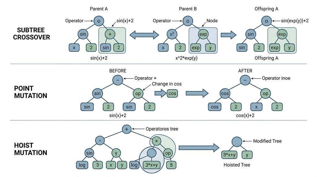
The standard GP loop has five phases per generation, shown in Figure 35.2:

1. Initialization. Generate a random population of \(P\) expression trees, typically using either the "full" method (all branches have the same depth) or the "grow" method (branches can terminate at different depths). The "ramped half-and-half" method alternates between full and grow at varying depths to produce a diverse initial population.
2. Evaluation. Compute the fitness (e.g., mean squared error (MSE) plus complexity penalty) of each individual on the training data.
3. Selection. Choose parents for the next generation based on fitness, using tournament selection, fitness-proportionate selection, or lexicographic selection.
4. Variation. Apply crossover (exchange subtrees between parents) and mutation (randomly modify subtrees) to produce offspring.
5. Replacement. Form the next generation from offspring, possibly retaining the best individual from the previous generation (elitism).

import numpy as np
import copy
from typing import Optional

# Use the Node class from Section 35.1 (Listing 35.1)

BINARY_OPS = ['+', '-', '*', '/']
UNARY_OPS = ['sin', 'cos']
ALL_OPS = BINARY_OPS + UNARY_OPS

def random_tree(max_depth: int, variables: list[str],
                const_range: tuple = (-5.0, 5.0),
                p_terminal: float = 0.3) -> 'Node':
    """Generate a random expression tree using the 'grow' method.

    At each internal position, randomly choose an operator.
    Terminate with a leaf (variable or constant) with probability p_terminal
    or when max_depth is reached.
    """
    if max_depth <= 0 or (max_depth > 1 and np.random.random() < p_terminal):
        # Leaf node: variable or constant
        if np.random.random() < 0.6:
            name = np.random.choice(variables)
            return Node(name, 0, [])
        else:
            val = np.random.uniform(*const_range)
            return Node(f'{val:.3f}', 0, [], value=val)

    op = np.random.choice(ALL_OPS)
    if op in BINARY_OPS:
        left = random_tree(max_depth - 1, variables, const_range, p_terminal)
        right = random_tree(max_depth - 1, variables, const_range, p_terminal)
        return Node(op, 2, [left, right])
    else:
        child = random_tree(max_depth - 1, variables, const_range, p_terminal)
        return Node(op, 1, [child])


def collect_nodes(tree: 'Node') -> list[tuple['Node', Optional['Node'], int]]:
    """Collect all (node, parent, child_index) triples in the tree."""
    result = [(tree, None, -1)]
    stack = [(tree, None, -1)]
    while stack:
        node, parent, idx = stack.pop()
        for i, child in enumerate(node.children):
            result.append((child, node, i))
            stack.append((child, node, i))
    return result


def subtree_crossover(parent1: 'Node', parent2: 'Node') -> 'Node':
    """Create offspring by replacing a random subtree of parent1
    with a random subtree from parent2."""
    offspring = copy.deepcopy(parent1)
    donor = copy.deepcopy(parent2)

    # Collect all nodes in both trees
    offspring_nodes = collect_nodes(offspring)
    donor_nodes = collect_nodes(donor)

    # Pick a random crossover point in the offspring (skip root for safety)
    if len(offspring_nodes) < 2:
        return offspring
    _, o_parent, o_idx = offspring_nodes[np.random.randint(1, len(offspring_nodes))]

    # Pick a random subtree from the donor
    d_node, _, _ = donor_nodes[np.random.randint(len(donor_nodes))]

    # Swap the subtree
    o_parent.children[o_idx] = d_node
    return offspring


def point_mutation(tree: 'Node', variables: list[str],
                   p_mutate: float = 0.1) -> 'Node':
    """Mutate individual nodes with probability p_mutate.

    Operators are replaced with operators of the same arity.
    Variables are replaced with other variables or constants.
    """
    tree = copy.deepcopy(tree)
    nodes = collect_nodes(tree)

    for node, parent, idx in nodes:
        if np.random.random() > p_mutate:
            continue
        if node.arity == 2:
            node.op = np.random.choice(BINARY_OPS)
        elif node.arity == 1:
            node.op = np.random.choice(UNARY_OPS)
        else:
            # Leaf: replace with a different variable or constant
            if np.random.random() < 0.6:
                node.op = np.random.choice(variables)
                node.value = None
            else:
                node.value = np.random.uniform(-5, 5)
                node.op = f'{node.value:.3f}'

    return tree


def hoist_mutation(tree: 'Node') -> 'Node':
    """Replace tree with one of its own subtrees (reduces complexity)."""
    nodes = collect_nodes(tree)
    # Pick a random internal node's child as the new root
    internal = [(n, p, i) for n, p, i in nodes if n.arity > 0 and p is not None]
    if not internal:
        return copy.deepcopy(tree)
    chosen, _, _ = internal[np.random.randint(len(internal))]
    return copy.deepcopy(chosen)

2. Tournament Selection

Tournament selection is the most widely used selection method in GP because it is simple, has tunable selection pressure, and does not require global fitness sorting. To select one parent, draw \(k\) individuals uniformly at random from the population, then choose the individual with the best fitness. The parameter \(k\) (the tournament size) controls selection pressure: \(k = 2\) gives gentle pressure (slightly favoring better individuals), while \(k = 7\) or higher gives aggressive pressure (strongly favoring the best).

A subtlety: tournament selection based on fitness alone can eliminate diversity too quickly, causing the population to converge to a single expression that is then unable to escape its local optimum. Lexicographic tournament selection addresses this by first comparing on fitness and then, among individuals with similar fitness (within a tolerance \(\epsilon\)), preferring the simpler one. This naturally maintains a Pareto front (the set of solutions where no other solution is simultaneously better on both accuracy and simplicity, introduced in Section 35.1) without requiring an explicit multi-objective framework.

import numpy as np

def tournament_select(population: list[dict], tournament_size: int = 5,
                      epsilon: float = 0.01) -> dict:
    """Lexicographic tournament selection.

    Among tournament participants, pick the one with best fitness.
    Among those within epsilon of the best, prefer the simplest.
    """
    # Draw tournament participants
    indices = np.random.choice(len(population), size=tournament_size, replace=False)
    participants = [population[i] for i in indices]

    # Find best fitness in tournament
    best_fitness = min(p['fitness'] for p in participants)

    # Among near-best, prefer simplest
    near_best = [p for p in participants
                 if p['fitness'] <= best_fitness * (1 + epsilon)]
    winner = min(near_best, key=lambda p: p['complexity'])

    return winner


def run_gp(X: np.ndarray, y: np.ndarray, variables: list[str],
           pop_size: int = 500, generations: int = 50,
           tournament_size: int = 5, p_crossover: float = 0.7,
           max_depth: int = 6, elite_size: int = 5) -> list[dict]:
    """Run a complete GP loop and return the Pareto front.

    Returns a list of dicts with keys: 'tree', 'fitness', 'complexity', 'mse'.
    """
    # Initialize population
    population = []
    for _ in range(pop_size):
        tree = random_tree(max_depth=max_depth, variables=variables)
        population.append({'tree': tree})

    best_ever = None
    data = {v: X[:, i] for i, v in enumerate(variables)}

    for gen in range(generations):
        # Evaluate fitness
        for ind in population:
            try:
                pred = ind['tree'].evaluate(data)
                mse = np.mean((pred - y) ** 2)
                if not np.isfinite(mse):
                    mse = 1e10
            except Exception:
                mse = 1e10
            complexity = ind['tree'].count_nodes()
            ind['mse'] = mse
            ind['complexity'] = complexity
            ind['fitness'] = mse  # pure fitness; Pareto handles complexity

        # Track best
        gen_best = min(population, key=lambda p: p['mse'])
        if best_ever is None or gen_best['mse'] < best_ever['mse']:
            best_ever = gen_best
        if gen % 10 == 0:
            print(f"Gen {gen:3d} | Best MSE: {gen_best['mse']:.6f} "
                  f"| Nodes: {gen_best['complexity']} "
                  f"| {gen_best['tree'].to_string()[:60]}")

        # Elitism: carry forward top individuals
        sorted_pop = sorted(population, key=lambda p: p['fitness'])
        new_population = [{'tree': copy.deepcopy(ind['tree'])}
                          for ind in sorted_pop[:elite_size]]

        # Breed offspring
        while len(new_population) < pop_size:
            if np.random.random() < p_crossover:
                p1 = tournament_select(population, tournament_size)
                p2 = tournament_select(population, tournament_size)
                child_tree = subtree_crossover(p1['tree'], p2['tree'])
            else:
                parent = tournament_select(population, tournament_size)
                # Choose mutation type
                r = np.random.random()
                if r < 0.6:
                    child_tree = point_mutation(parent['tree'], variables)
                elif r < 0.8:
                    child_tree = hoist_mutation(parent['tree'])
                else:
                    child_tree = random_tree(max_depth, variables)

            # Depth limit: reject trees that are too deep
            if child_tree.count_nodes() <= 50:
                new_population.append({'tree': child_tree})

        population = new_population

    # Compute final Pareto front
    for ind in population:
        try:
            pred = ind['tree'].evaluate(data)
            ind['mse'] = float(np.mean((pred - y) ** 2))
            if not np.isfinite(ind['mse']):
                ind['mse'] = 1e10
        except Exception:
            ind['mse'] = 1e10
        ind['complexity'] = ind['tree'].count_nodes()
        ind['expr'] = ind['tree'].to_string()

    return pareto_front([{'expr': ind['expr'], 'mse': ind['mse'],
                          'complexity': ind['complexity']}
                        for ind in population if ind['mse'] < 1e9])

3. Neural-Guided Symbolic Regression

Classical GP treats expression search as a purely evolutionary process: no mathematical knowledge guides the operators. A crossover between \(\sin(x)\) and \(\exp(y)\) is as likely as a crossover between \(x^2\) and \(x^3\), even though the latter is more likely to be useful if the true expression is a polynomial, since the two parents already share a compatible algebraic structure. Neural-guided symbolic regression uses trained neural networks to inject mathematical knowledge into the search, either by directly generating candidate expressions or by steering evolutionary operators toward promising regions.

Three architectures have emerged as dominant paradigms, each representing a different way to combine neural networks with symbolic search. The first two (transformer generation and reinforcement learning) replace GP's blind operators with learned ones; the third (hybrid approaches, including PySR's integration with LLMs) keeps the evolutionary backbone and uses neural networks to warm-start or steer the population.

3.1 Transformer-Based Expression Generation

The most direct approach treats symbolic regression as a sequence-to-sequence translation problem. A transformer encoder processes the input dataset (a set of \((x, y)\) pairs), and a transformer decoder generates an expression token by token in prefix notation (where each operator precedes its arguments, so \(+ \; * \; x \; y \; z\) represents \(x \cdot y + z\)). Kamienny et al. (2022) trained such a model on millions of synthetic equation-dataset pairs, producing a system that can generate candidate expressions in a single forward pass, without any evolutionary search.

The key insight is that the encoder must handle a set of data points (the order of \((x_i, y_i)\) pairs should not matter), while the decoder must produce a sequence of expression tokens. The encoder uses a set-transformer architecture (a variant of the transformer designed to process unordered sets rather than sequences, using learned "inducing points" to summarize the input set efficiently) (Lee et al., 2019) that is permutation-invariant over data points, while the decoder is a standard autoregressive transformer (generating one token at a time, each conditioned on all previously emitted tokens) with causal masking.

import numpy as np

# Pseudocode for transformer-based symbolic regression
# (Full implementation requires PyTorch; this shows the architecture)

class SymbolicTransformer:
    """End-to-end symbolic regression with a transformer.

    Architecture:
      1. Encoder: Set-Transformer over (x, y) pairs
         - Input: N data points, each a (d+1)-dimensional vector [x_1,...,x_d, y]
         - Permutation-invariant via induced set attention (ISAB)
         - Output: fixed-size latent representation z

      2. Decoder: Autoregressive transformer
         - Input: z (from encoder) + previously generated tokens
         - Output: probability distribution over next token
         - Vocabulary: operators (+, -, *, /, sin, cos, exp, log, sqrt)
                       variables (x_1, ..., x_d)
                       constants (discretized or placeholder)
         - Generates expression in prefix notation: + * x1 x1 1.0 => x1^2 + 1
    """

    def encode_dataset(self, X, y):
        """Encode a dataset of (x, y) pairs into a latent vector.

        Uses Induced Set Attention Blocks (ISAB) for permutation invariance.
        The encoder sees the DATA, not any symbolic representation.
        """
        # Stack inputs and outputs: each point is [x_1, ..., x_d, y]
        data_points = np.column_stack([X, y])
        # ... Set-Transformer encoder produces latent z
        return "latent_z"  # placeholder

    def decode_expression(self, z, max_tokens=50):
        """Autoregressively generate expression tokens.

        At each step:
          1. Feed z and all previously generated tokens to the decoder
          2. Sample the next token from the output distribution
          3. Stop when  is generated or max_tokens is reached

        Temperature controls exploration vs. exploitation:
          - Low temperature (0.1): greedy, picks highest-probability tokens
          - High temperature (1.0): diverse, explores alternative expressions
        """
        tokens = []
        for _ in range(max_tokens):
            # next_token = decoder(z, tokens)
            # tokens.append(next_token)
            # if next_token == '': break
            pass
        return tokens

    def beam_search(self, z, beam_width=10):
        """Generate multiple candidate expressions via beam search.

        Maintains beam_width partial expressions at each step,
        expanding each by its top-k next tokens, then pruning to
        the beam_width most probable sequences.

        Returns beam_width complete expressions ranked by probability.
        """
        pass

# Training procedure (conceptual):
# 1. Generate millions of random symbolic expressions
# 2. For each expression, sample N data points to create a dataset
# 3. Train the transformer to predict the expression from the dataset
# 4. At inference, encode the real dataset and decode candidate expressions

The transformer approach has a remarkable property: at inference time, it requires only a single forward pass through the network (or a beam search, which maintains the top-\(k\) most probable partial sequences at each decoding step, with a few passes) rather than the thousands of evaluations needed by evolutionary search. On the SRBench benchmark (La Cava et al., 2021, covering 122 regression problems), transformer models tend to match or exceed GP on problems with clean data and known functional forms. However, they generally struggle with noisy data and out-of-distribution expressions (functions unlike anything seen during training), where evolutionary methods remain more robust.

3.2 Reinforcement Learning for Expression Construction

An alternative to supervised training on synthetic data is to frame expression construction as a sequential decision-making problem. At each step, an agent chooses the next token in a prefix- notation expression. The reward is the negative of the expression's fitness (MSE plus complexity penalty) when the expression is complete. The agent learns a policy that maximizes expected reward, effectively learning which operator sequences tend to produce good fits.

Petersen et al. (2021) introduced Deep Symbolic Regression (DSR) using this framework. The agent is a recurrent neural network (RNN) that maintains a hidden state summarizing the partial expression built so far. At each step, it outputs a distribution over the token vocabulary, samples a token, and appends it to the expression. When the expression is syntactically complete (the tree has no unfilled slots), the agent receives a reward based on how well the expression fits the data.

The critical innovation in DSR is the risk-seeking policy gradient. Standard policy gradient methods (REINFORCE, the foundational algorithm that estimates the gradient of expected reward from sampled trajectories) optimize the expected reward. But in symbolic regression, we do not care about average performance across sampled expressions; we care about the best single expression found. DSR uses a quantile-based objective that focuses the gradient on the top \(\epsilon\)-fraction of sampled expressions, concentrating learning on the rare high-reward trajectories:

where \(R_{1-\epsilon}\) is the \((1-\epsilon)\)-quantile of rewards in the current batch and \(\mathbf{1}[\cdot]\) is the indicator function. Only trajectories (expressions) with reward above this threshold contribute to the gradient update, which dramatically improves convergence for the rare-reward structure of symbolic regression.

Mental Model

Think of the risk-seeking policy gradient as a talent-show judge who only remembers the best acts. Imagine a cooking competition where 1,000 contestants each prepare a dish. A standard judge would average all the scores, conclude that the typical dish was mediocre, and give broad feedback like "use more salt." The risk-seeking judge ignores the bottom 950 dishes entirely and studies only the top 50, asking: what did these winners do differently? The feedback becomes specific and actionable: "the winners all used a citrus glaze on the protein." In the same way, the risk-seeking gradient ignores the vast majority of poorly fitting expressions and concentrates the learning signal on the rare few that achieved high reward, extracting the structural patterns (operator choices, variable combinations) that made those expressions successful.

import numpy as np

def risk_seeking_policy_gradient(
    log_probs: np.ndarray,   # log probability of each sampled expression
    rewards: np.ndarray,     # reward (negative fitness) of each expression
    epsilon: float = 0.05    # top fraction to focus on
) -> np.ndarray:
    """Compute the risk-seeking policy gradient for symbolic regression.

    Instead of optimizing expected reward (standard REINFORCE), focus the
    gradient on the top epsilon-fraction of sampled expressions.

    Args:
        log_probs: shape (batch_size,), log pi(expression_i)
        rewards: shape (batch_size,), reward for each expression
        epsilon: fraction of top-performing expressions to learn from

    Returns:
        gradient: weighted log-prob gradient for the policy update
    """
    # Find the (1-epsilon) quantile of rewards
    quantile_threshold = np.quantile(rewards, 1 - epsilon)

    # Mask: only include expressions above the threshold
    mask = rewards >= quantile_threshold

    # Advantage: how much better than the threshold
    advantages = (rewards - quantile_threshold) * mask

    # Normalize advantages for stable gradients
    if advantages.sum() > 0:
        advantages = advantages / (advantages.std() + 1e-8)

    # Policy gradient: high-reward expressions get positive gradient
    gradient = log_probs * advantages

    n_selected = mask.sum()
    print(f"Risk-seeking: {n_selected}/{len(rewards)} expressions "
          f"above quantile {quantile_threshold:.4f}")

    return gradient


# Example: batch of 1000 sampled expressions
np.random.seed(42)
n_batch = 1000
fake_log_probs = np.random.normal(-5, 2, n_batch)  # typical log probs
fake_rewards = np.random.exponential(0.1, n_batch)  # most are bad

# Inject a few good expressions (realistic: rare high-reward events)
fake_rewards[42] = 5.0   # excellent fit
fake_rewards[137] = 4.2  # very good fit
fake_rewards[500] = 3.8  # good fit

grad = risk_seeking_policy_gradient(fake_log_probs, fake_rewards, epsilon=0.05)
# Risk-seeking: 50/1000 expressions above quantile 0.2750

4. PySR: Multi-Population Evolutionary Search

Transformer generation and reinforcement learning both show that learned mathematical priors accelerate symbolic search, yet each has a cost: transformers need massive pretraining corpora, and RL agents train slowly on one dataset at a time. Can these neural insights fold into the evolutionary backbone that already handles diversity and robustness?

PySR (Cranmer, 2023) represents the current state of the art for practical symbolic regression. It combines classical GP with several innovations that address the weaknesses of both pure evolutionary and pure neural approaches. PySR's architecture reappears in Section 35.3, where it forms the core of the discovery pipeline.

PySR's key design decisions:

1. Multi-population island model. Instead of one large population, PySR runs \(M\) independent populations (typically 20 to 40) that evolve in parallel. Periodically, the best individual from one population migrates to another. This maintains diversity (each island can explore a different region of expression space) while allowing good solutions to spread across the ensemble. It is the evolutionary analog of ensemble methods in machine learning.
2. Adaptive complexity weighting. Rather than a fixed parsimony coefficient (a penalty multiplier applied to expression complexity, so that fitness = MSE + parsimony * node_count), PySR uses a temperature-based scheme that periodically increases complexity penalties (cooling) and decreases them (heating). During hot phases, complex expressions are tolerated, allowing the search to explore elaborate structures. During cold phases, complexity is heavily penalized, pruning away bloat and favoring simple expressions. This annealing schedule prevents the search from getting stuck in either regime.
3. Constant optimization. After each generation, PySR optimizes the numerical constants in each expression using BFGS (a quasi-Newton method from scipy.optimize). This is critical: GP is good at discovering the structure of an expression (\(a \cdot x^2 + b\)) but poor at finding precise constant values (\(0.5 \cdot x^2 + 1.0\)). By separating structure search (GP) from constant fitting (BFGS), PySR gets the best of both approaches.

4. Julia backend. PySR's core engine is written in Julia (SymbolicRegression.jl), which provides near-C performance for expression evaluation. The Python wrapper handles I/O and visualization. This architecture typically means PySR runs 10 to 100x faster than pure-Python GP implementations (as of 2024, the legacy gplearn library is no longer actively maintained; PySR and the newer FEAT library are the primary Python-accessible SR tools).

from pysr import PySRRegressor
import numpy as np

# PySR configuration for a physics problem
model = PySRRegressor(
    # Search configuration
    niterations=100,           # number of evolutionary cycles
    populations=30,            # number of independent island populations
    population_size=50,        # individuals per population
    ncycles_per_iteration=300, # inner cycles per iteration (Julia-side)

    # Operator vocabulary
    binary_operators=["+", "-", "*", "/", "^"],
    unary_operators=["sin", "cos", "exp", "log", "sqrt", "abs"],

    # Complexity control
    maxsize=30,                # maximum expression tree size (nodes)
    maxdepth=8,                # maximum tree depth
    parsimony=0.0032,          # adaptive complexity penalty base
    adaptive_parsimony_scaling=1000.0,  # temperature for adaptive penalty

    # Constant optimization
    optimizer_algorithm="BFGS",     # quasi-Newton for constant fitting
    optimizer_nrestarts=3,          # random restarts for constant optimization
    optimize_probability=0.14,      # fraction of individuals that get constant opt

    # Batching and performance
    batching=True,             # subsample data per evaluation (faster)
    batch_size=50,             # subsample size

    # Output
    equation_file="hall_of_fame.csv",  # save Pareto front to CSV
    progress=True,
    verbosity=1,
    random_state=42,
)

# Example: recover the ideal gas law PV = nRT
# Variables: P (pressure), V (volume), n (moles), T (temperature)
# Target: PV/nT should be approximately R = 8.314
np.random.seed(42)
n_points = 200
P = np.random.uniform(1e4, 1e6, n_points)     # Pa
V = np.random.uniform(0.001, 0.1, n_points)    # m^3
n_mol = np.random.uniform(0.1, 10.0, n_points) # mol
T = np.random.uniform(200, 500, n_points)       # K
R = 8.314  # J/(mol*K)

# Target: P = nRT/V (rearranged ideal gas law)
y = n_mol * R * T / V + np.random.normal(0, 100, n_points)  # noisy pressure

X = np.column_stack([V, n_mol, T])

model.fit(X, y, variable_names=["V", "n", "T"])

# Display the Pareto front of discovered equations
print("\nPareto front (complexity vs. loss):")
print(model)
# Typical output (exact results vary by run):
# Complexity | Loss       | Equation
# 1          | 3.24e+10   | 336820.0
# 3          | 1.82e+08   | (T * 164.85)
# 5          | 2.41e+06   | ((n * T) * 85.43)
# 7          | 9847.2     | ((n * T) / V) * 8.317
# 9          | 9841.6     | ((n * (T + 0.182)) / V) * 8.314

5. Scaling Challenges and Hybrid Approaches

PySR's combination of island migration, adaptive parsimony, and constant optimization makes it the strongest single tool available today, but even its multi-population architecture cannot outrun the combinatorial explosion that awaits as problem dimensionality grows.

All symbolic regression methods face a fundamental scaling wall: the number of possible expressions grows super-exponentially with the number of input variables. For \(d\) input variables, \(k\) operators, and expressions of size \(n\), the number of distinct trees scales roughly as \((2k + d)^n\). With \(d = 20\) variables and \(n = 15\) nodes, this exceeds \(10^{20}\), more candidate expressions than there are grains of sand on Earth.

Taming the Combinatorial Explosion

Several strategies address this scaling challenge. Feature selection reduces \(d\) before symbolic regression begins, using mutual information or gradient-based importance from Chapter 25. Modular decomposition (used in AI Feynman) searches for separability (\(f(x,y) = g(x) + h(y)\) or \(f(x,y) = g(x) \cdot h(y)\)) and solves the subproblems independently. Hybrid neural-evolutionary approaches use a neural network as a warm-start for the evolutionary search: the transformer generates an initial population of plausible expressions, then GP refines them through crossover and mutation.

The most promising recent direction combines large language models (LLMs) with symbolic regression. LLMs can propose candidate functional forms based on natural-language descriptions of the problem domain ("this data describes a damped oscillator"), which are then refined by PySR. This connects symbolic regression to the hypothesis generation systems of Chapter 39 and the AI scientist architectures of Chapter 53, where LLMs serve as the creative hypothesis engine and symbolic regression provides the rigorous mathematical verification.

Exercises

1. (Conceptual) Compare and contrast three approaches to symbolic regression: (a) genetic programming, (b) transformer-based generation, and (c) reinforcement learning. For each, identify: the search strategy, the training signal, the main computational bottleneck, and the failure mode. Which approach would you choose for (i) a physics problem with 3 variables and known dimensions, and (ii) a biology problem with 50 features and no dimensional information?
2. (Coding) Implement a simple "island model" by running the run_gp function from Listing 35.7 with 4 independent populations of 200 individuals each. Every 10 generations, migrate the best individual from each population to the next (circular topology). Compare the final Pareto front to a single population of 800 individuals. Does the island model find better or more diverse solutions?
3. (Analysis) Using PySR (Listing 35.10), fit the dataset generated by \(y = 3.0 \cdot \sin(2\pi x_1) + x_2^2\) with 500 data points and Gaussian noise \(\sigma \in \{0.01, 0.1, 1.0, 5.0\}\). For each noise level, report the complexity of the best expression on the Pareto front and whether the correct functional form is recovered. At what noise level does symbolic regression begin to fail?