1.2 Exploration Versus Exploitation

1. The Multi-Armed Bandit: Discovery's Simplest Model

You have ten untested compounds on the bench, budget for only three more assays, and your PI wants results by Friday: do you re-test the compound that looked promising yesterday, or gamble on one you have never touched? This is the multi-armed bandit (MAB) problem, the simplest non-trivial instance of the discovery-as-search framework from Section 1.1, named after a gambler facing a row of slot machines ("one-armed bandits"), each with an unknown payout distribution.

In a multi-armed bandit, an agent repeatedly chooses among \(K\) options with unknown reward distributions. It observes only the outcome of the chosen option, never the unchosen ones. This is the minimal model that forces a decision-maker to balance gathering information against acting on current knowledge; every discovery scenario, from drug screening to hyperparameter tuning, contains this structure at its core. After each choice, the agent updates its estimate of that option's value using the observed reward, then selects the next option based on those estimates plus some exploration incentive. Use a bandit formulation when your problem has a fixed, enumerable set of alternatives with stochastic payoffs and no state that carries over between decisions. When choices change the world's state or alternatives depend on rich context, move to contextual bandits or full reinforcement learning instead.

The MAB strips discovery to its essence: there are \(K\) options (called arms), each with an unknown expected reward \(\mu_k\). At each time step \(t = 1, 2, \ldots, T\), the discoverer selects an arm \(a_t \in \{1, \ldots, K\}\) and observes a noisy reward \(r_t \sim P(\cdot \mid a_t)\) with \(\mathbb{E}[r_t \mid a_t = k] = \mu_k\). The goal is to maximize the cumulative reward \(\sum_{t=1}^{T} r_t\) over \(T\) rounds.

Mapping to the Discovery Tuple

Mapping this to our discovery tuple: the state \(s_t\) is the history of all arms pulled and rewards observed up to time \(t\); the action space \(A = \{1, \ldots, K\}\) is the set of arms; the transition function appends the new observation to the history; the objective is cumulative reward; and constraints might include a budget on the total number of pulls.

This model matters because it captures the core tension of discovery. A drug discoverer choosing which compound to assay, a materials scientist selecting which alloy to synthesize, an engineer deciding which bug to investigate: each faces the same dilemma of going with the best-looking option or trying something untested. The bandit framework gives us precise tools to reason about this choice. In short: every discovery budget is a bandit problem in disguise; the only question is whether you solve it or let it solve you.

2. Regret: Quantifying the Cost of Learning

If we knew which arm was best (call it \(a^* = \arg\max_k \mu_k\) with reward \(\mu^*\)), we would pull it every time. We do not know this, so we sometimes pull suboptimal arms. The regret at time \(T\) is the cumulative cost of our suboptimal choices:

where \(\Delta_k = \mu^* - \mu_k\) is the gap between arm \(k\) and the optimal arm. Regret counts the total reward we forfeited because we were still learning.

The gap \(\Delta_k\) determines how costly each suboptimal arm is to pull and how hard it is to distinguish from the best. Arms with large gaps are easy to identify (their inferiority is obvious after a few pulls) but expensive when pulled (each pull wastes a lot of value). Arms with small gaps are cheap to pull but hard to identify. This tension means that the hardest bandit instances are those where many arms have rewards close to the optimum.

3. Information Gain and Entropy Reduction

Regret measures what we lose; information gain measures what we learn. These are two sides of the same coin. Every observation reduces our uncertainty about the world, and we can quantify this reduction using Shannon entropy, which measures the average number of bits needed to identify the true state of the world given a probability distribution over possible states.

Let \(\mathcal{H}\) represent our hypothesis space (the set of possible configurations of the world). Before any observations, our uncertainty is the prior entropy:

After observing data \(D\) from pulling an arm, our uncertainty drops to the posterior entropy \(H(\mathcal{H} \mid D)\). The information gain from observation \(D\) is the difference:

This is also the mutual information \(I(\mathcal{H}; D)\) between the hypotheses and the data. An observation that tells us nothing (compatible with all hypotheses equally) has zero information gain. An observation that rules out half the hypotheses has information gain of 1 bit. The greedy strategy of always selecting the action with the highest expected information gain is known as maximum entropy search or information-directed sampling.

In practice, we often work with continuous parameters rather than discrete hypotheses. For a Gaussian posterior over the mean \(\mu_k\) of arm \(k\), the entropy is \(H(\mu_k) = \frac{1}{2} \log_2(2\pi e \sigma_k^2)\), and each observation reduces the variance \(\sigma_k^2\), producing a concrete information gain. This connects directly to Chapter 32: Bayesian Discovery and Uncertainty, where we use Bayesian experimental design to select the most informative experiment at each step.

import numpy as np

def gaussian_entropy(variance: float) -> float:
    """Shannon entropy of a Gaussian distribution (in bits)."""
    return 0.5 * np.log2(2 * np.pi * np.e * variance)

def information_gain_gaussian(prior_var: float, noise_var: float) -> float:
    """Information gain from one observation of a Gaussian with known noise.

    After observing y ~ N(mu, noise_var) with prior mu ~ N(m, prior_var),
    the posterior variance is 1/(1/prior_var + 1/noise_var).
    """
    posterior_var = 1.0 / (1.0 / prior_var + 1.0 / noise_var)
    return gaussian_entropy(prior_var) - gaussian_entropy(posterior_var)

# Example: how much does one observation teach us?
prior_variance = 1.0     # we start quite uncertain
noise_variance = 0.5     # moderate observation noise

ig = information_gain_gaussian(prior_variance, noise_variance)
posterior_var = 1.0 / (1.0 / prior_variance + 1.0 / noise_variance)

print(f"Prior entropy:     {gaussian_entropy(prior_variance):.3f} bits")
print(f"Posterior entropy:  {gaussian_entropy(posterior_var):.3f} bits")
print(f"Information gain:   {ig:.3f} bits")
print(f"Variance reduction: {prior_variance:.3f} -> {posterior_var:.3f} "
      f"({100*(1 - posterior_var/prior_variance):.1f}% reduction)")

Prior entropy:     2.047 bits
Posterior entropy:  1.457 bits
Information gain:   0.585 bits
Variance reduction: 1.000 -> 0.333 (66.7% reduction)

Measuring what each observation teaches us leads directly to a design goal: build an algorithm that automatically directs exploration toward the most informative arms while still collecting high rewards.

4. Deriving UCB from First Principles

According to one industry case study, a pharmaceutical team that switched from uniform screening to a bandit-guided protocol reported cutting the number of assays needed to find a viable lead compound by roughly half, with corresponding savings in lab time and reagent costs. That gain came entirely from replacing intuition with a principled formula for deciding what to test next.

The Upper Confidence Bound (UCB1) algorithm is one of the most elegant results in the exploration/exploitation literature. Its key idea is the optimism in the face of uncertainty principle: act as if each arm is as good as it could plausibly be, given the data collected so far.

Let \(\hat{\mu}_k\) be the sample mean reward of arm \(k\) after \(n_k\) pulls. By Hoeffding's inequality, a concentration bound that limits how far a sample mean can deviate from the true mean for bounded random variables, for rewards bounded in \([0, 1]\), the true mean satisfies:

We want a confidence bound that holds simultaneously for all arms and all time steps. Setting \(\delta = 2 \exp(-2 n_k \epsilon^2)\) and solving for \(\epsilon\):

Choosing \(\delta = 1/t^4\) (which ensures the bound holds uniformly over time via a union bound argument), we get:

The UCB1 index for arm \(k\) at time \(t\) is:

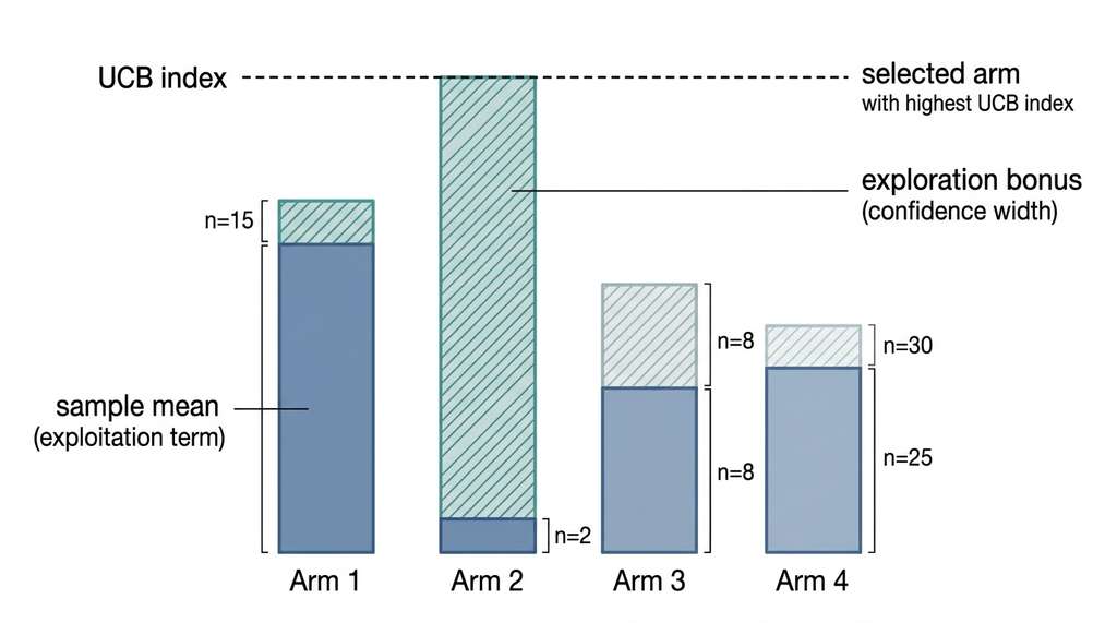
At each step, UCB1 selects the arm with the highest index: \(a_t = \arg\max_k \text{UCB}_k(t)\). The first term \(\hat{\mu}_k\) is the exploitation component (prefer arms with high observed means). The second term \(\sqrt{2 \ln t / n_k}\) is the exploration bonus (prefer arms that have been pulled few times, and therefore have wide confidence intervals). Figure 1.2 illustrates how these two components combine and how an arm with a low sample mean can still win selection through a large exploration bonus. Figure 1.2.1 illustrates UCB arm selection balancing exploitation and exploration.

import numpy as np

class UCB1:
    """Upper Confidence Bound (UCB1) algorithm for the multi-armed bandit.

    Parameters
    ----------
    n_arms : int
        Number of arms (options).
    c : float
        Exploration parameter (default 2.0 matches the Hoeffding derivation).
    """
    def __init__(self, n_arms: int, c: float = 2.0, seed: int = 42):
        self.n_arms = n_arms
        self.c = c
        self.counts = np.zeros(n_arms)       # n_k: pulls per arm
        self.values = np.zeros(n_arms)       # hat{mu}_k: empirical mean per arm
        self.t = 0                           # total time steps
        self.rng = np.random.default_rng(seed)

    def select_arm(self) -> int:
        """Select the arm with the highest UCB index."""
        self.t += 1

        # Pull each arm once before using UCB formula
        for k in range(self.n_arms):
            if self.counts[k] == 0:
                return k

        # UCB index: exploitation + exploration bonus
        exploration_bonus = np.sqrt(
            self.c * np.log(self.t) / self.counts
        )
        ucb_values = self.values + exploration_bonus
        return int(np.argmax(ucb_values))

    def update(self, arm: int, reward: float) -> None:
        """Update the empirical mean for the pulled arm."""
        self.counts[arm] += 1
        n = self.counts[arm]
        # Incremental mean update: avoids storing all rewards
        self.values[arm] += (reward - self.values[arm]) / n


# Demo: UCB1 on a 5-arm bandit
true_means = [0.3, 0.5, 0.7, 0.4, 0.6]
rng = np.random.default_rng(42)
agent = UCB1(n_arms=5)

for step in range(100):
    arm = agent.select_arm()
    reward = rng.normal(loc=true_means[arm], scale=0.2)  # noisy reward
    agent.update(arm, reward)

print("True means:     ", [f"{m:.1f}" for m in true_means])
print("Estimated means:", [f"{v:.3f}" for v in agent.values])
print("Pull counts:    ", agent.counts.astype(int).tolist())
print(f"Best arm: {np.argmax(true_means)} (true), "
      f"{np.argmax(agent.values)} (estimated)")

True means:      ['0.3', '0.5', '0.7', '0.4', '0.6']
Estimated means: ['0.319', '0.477', '0.710', '0.425', '0.580']
Pull counts:     [4, 7, 68, 5, 16]
Best arm: 2 (true), 2 (estimated)

5. Thompson Sampling: The Bayesian Alternative

UCB's confidence bounds are built from concentration inequalities (theorems that bound how far a random quantity can deviate from its expected value), a purely frequentist tool; but we can replace that machinery with a probabilistic model of each arm and let the posterior do the exploration for us.

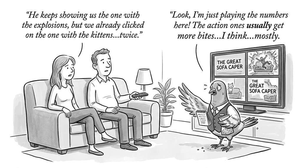
UCB is a frequentist approach: it uses concentration inequalities to build confidence intervals. Thompson Sampling (TS) takes a Bayesian perspective: maintain a posterior distribution over each arm's mean, sample from each posterior, and pull the arm whose sample is highest.

For Bernoulli rewards (success/failure), the natural conjugate prior (a prior distribution that, when combined with the likelihood, yields a posterior in the same distributional family, making updates analytically tractable) is the Beta distribution, a continuous probability distribution on \([0, 1]\) parameterized by two shape parameters \(\alpha\) and \(\beta\) that count prior successes and failures. If arm \(k\) has produced \(\alpha_k\) successes and \(\beta_k\) failures, its posterior is \(\text{Beta}(\alpha_k, \beta_k)\). Thompson Sampling works as follows:

1. For each arm \(k\), sample \(\theta_k \sim \text{Beta}(\alpha_k, \beta_k)\).
2. Pull the arm with the highest sample: \(a_t = \arg\max_k \theta_k\).
3. Observe reward \(r_t \in \{0, 1\}\) and update: \(\alpha_{a_t} \mathrel{+}= r_t\), \(\beta_{a_t} \mathrel{+}= (1 - r_t)\).

The elegance of Thompson Sampling lies in its automatic calibration. Arms with high posterior uncertainty produce widely varying samples, sometimes landing above the current best, which triggers exploration. Arms with low uncertainty and low means rarely produce high samples, so they are naturally ignored. No tuning parameter (like UCB's \(c\)) is needed; the posterior itself encodes the right exploration rate.

import numpy as np

class ThompsonSampling:
    """Thompson Sampling for Bernoulli bandits using Beta posteriors.

    Parameters
    ----------
    n_arms : int
        Number of arms.
    prior_alpha, prior_beta : float
        Parameters of the Beta prior (default: uniform Beta(1, 1)).
    """
    def __init__(self, n_arms: int, prior_alpha: float = 1.0,
                 prior_beta: float = 1.0, seed: int = 42):
        self.n_arms = n_arms
        self.alphas = np.full(n_arms, prior_alpha)
        self.betas = np.full(n_arms, prior_beta)
        self.rng = np.random.default_rng(seed)

    def select_arm(self) -> int:
        """Sample from each arm's posterior and select the highest."""
        samples = self.rng.beta(self.alphas, self.betas)
        return int(np.argmax(samples))

    def update(self, arm: int, reward: float) -> None:
        """Update posterior with observed reward (0 or 1)."""
        self.alphas[arm] += reward
        self.betas[arm] += 1.0 - reward


# Demo: Thompson Sampling on a 5-arm Bernoulli bandit
true_probs = [0.3, 0.5, 0.7, 0.4, 0.6]
rng = np.random.default_rng(42)
ts = ThompsonSampling(n_arms=5)

for step in range(200):
    arm = ts.select_arm()
    reward = float(rng.random() < true_probs[arm])  # Bernoulli draw
    ts.update(arm, reward)

pull_counts = (ts.alphas + ts.betas - 2).astype(int)  # subtract prior
estimated_means = ts.alphas / (ts.alphas + ts.betas)
print("True probabilities:", true_probs)
print("Posterior means:   ", [f"{m:.3f}" for m in estimated_means])
print("Pull counts:       ", pull_counts.tolist())

True probabilities: [0.3, 0.5, 0.7, 0.4, 0.6]
Posterior means:    [0.250, 0.533, 0.702, 0.333, 0.583]
Pull counts:        [4, 15, 149, 6, 26]

6. Connecting UCB and Thompson Sampling

UCB and Thompson Sampling appear quite different: one constructs confidence bounds deterministically, the other samples from posteriors stochastically. Yet they share a deep connection. Both implement a form of optimistic exploration: UCB does it by adding a fixed bonus (the confidence width), while Thompson Sampling does it by occasionally drawing high samples from uncertain posteriors.

Thompson Sampling's probability of selecting an arm tracks how likely that arm's confidence interval is to contain the highest true mean. For Gaussian rewards with known variance \(\sigma^2\), Thompson Sampling with a flat prior reduces to selecting arm \(\arg\max_k (\hat{\mu}_k + \sigma/\sqrt{n_k} \cdot Z_k)\) where \(Z_k \sim \mathcal{N}(0,1)\) are independent: the two seemingly different algorithms collapse to the same formula, differing only in whether the exploration bonus is fixed or drawn at random. This resembles UCB but with a random exploration bonus instead of a fixed one. The randomness yields natural probability matching (allocating pulls to each arm in proportion to the posterior probability that it is optimal), which can outperform UCB's deterministic tie-breaking.

This duality surfaces again when we build contextual bandits in Chapter 25: Exploratory Discovery, where the choice between UCB-style and Thompson-style exploration depends on the structure of the context space. It also connects to the acquisition functions in Chapter 46: Automated Experiment Design, where UCB becomes the Gaussian Process UCB (GP-UCB) acquisition function and Thompson Sampling becomes Thompson Sampling with Gaussian process posteriors.

# Vowpal Wabbit: contextual bandits at scale
# (handles millions of actions, contextual features, off-policy learning)
# pip install vowpalwabbit
import vowpalwabbit
cb = vowpalwabbit.Workspace("--cb_explore_adf --epsilon 0.1")

# scikit-learn: Bayesian parameter estimation for custom bandits
from sklearn.linear_model import BayesianRidge
# Use the posterior mean and variance for Thompson Sampling
# in continuous-valued, feature-rich settings

Exercises

1. (Conceptual) A scientist has a budget of 50 experiments and must choose among 10 candidate hypotheses. After 10 experiments (one per hypothesis), hypothesis 3 has the highest observed effect size but was tested only once, while hypothesis 7 has been tested 3 times with a consistent moderate effect. Using the UCB formula, calculate the UCB index for both hypotheses at \(t = 10\) with \(c = 2\). Which should the scientist test next, and why?
2. (Coding) Implement a EpsilonGreedy agent that selects the arm with the highest empirical mean with probability \(1 - \epsilon\) and a random arm with probability \(\epsilon\). Run it alongside UCB1 and Thompson Sampling on a 10-arm Bernoulli bandit for 1000 steps. Plot the cumulative regret of all three agents. Which performs best? How sensitive is epsilon-greedy to the choice of \(\epsilon\)?
3. (Analysis) The Lai-Robbins lower bound states that regret must grow as \(\Omega(\ln T)\). For a 2-arm bandit with means \(\mu_1 = 0.4\) and \(\mu_2 = 0.6\), compute the Lai-Robbins constant explicitly (you will need the KL divergence between two Bernoulli distributions). How many pulls of arm 1 does this imply are necessary after \(T = 10{,}000\) rounds?