1.3 Discovery Workflows

1. From Single Decisions to Sequential Workflows

A graduate student runs a promising experiment, gets an ambiguous result, redesigns the protocol, waits two weeks for new reagents, reruns the experiment, discovers a confound in the original data, and starts over from scratch: six months consumed, with the finish line no closer than it was on day one. The culprit is not any single slow step but the dependencies between steps. In Section 1.2 we modeled discovery as choosing among options at a single decision point, yet real discovery unfolds as a chain of decisions where each outcome determines which steps become available next. These dependencies create a workflow, a structured sequence of activities with conditional branching.

Without a formal model of the workflow, teams optimize the wrong stage: they pour resources into speeding up a 30-day experiment by 10% while ignoring a 14-day literature review that AI could potentially compress by 90%. The formalism below makes such misallocations visible before a single dollar is spent.

We formalize a discovery workflow as a state transition system (STS):

A state transition system is a mathematical model. It captures every configuration a process can occupy (its states), every action that moves the process between configurations (its transitions), and the rules governing which actions are legal in which states (its transition function). This matters because it converts an informal, ad hoc research process into a precise, analyzable object. Once a workflow is an STS, you can compute its critical path (the longest sequence of dependent transitions that determines the minimum total duration), identify bottlenecks, prove that every state is reachable, and program an AI agent to navigate it automatically. The mechanism is straightforward: at each moment the system occupies exactly one state. When an action fires, the transition function selects the next state (deterministically or stochastically), and the system moves there. Use an STS when the process has discrete, well-defined phases and you need to reason about sequencing, reachability, or cycle detection. For continuous processes without clear phase boundaries, a differential-equation or agent-based model may fit better.

where:

• \(Q\): A finite set of workflow states (not to be confused with the discovery states \(S\) from Section 1.1). Each workflow state represents a phase of the discovery process: "hypothesis formed," "experiment designed," "data collected," "analysis complete," and so on.
• \(q_0 \in Q\): The initial state (e.g., "problem identified").
• \(\Sigma\): The set of workflow actions (termed an "alphabet" in automata theory): transitions between phases. Actions include "design experiment," "run simulation," "analyze data," "revise model," "publish results."
• \(\delta: Q \times \Sigma \to Q\): The transition function, mapping a current phase and action to the next phase. For stochastic workflows, \(\delta: Q \times \Sigma \to \Delta(Q)\) (where \(\Delta(Q)\) denotes the set of probability distributions over \(Q\)) maps to a distribution over next states (an experiment might succeed or fail, leading to different phases).
• \(F \subseteq Q\): The set of terminal states representing successful discovery outcomes: a validated finding, a published result, a deployed innovation.

This formalism nests inside the discovery tuple from Section 1.1. The discovery-level state space \(S\) describes what has been discovered; the workflow-level state space \(Q\) describes where in the process the discoverer is. A complete description of the discovery at any moment combines both: the knowledge accumulated so far and the current workflow phase. The deterministic transition function used here suffices for structural analysis (critical paths, bottlenecks, reachability); stochastic transitions, where experimental outcomes are uncertain, become central in the simulation and Bayesian methods of Parts III and V.

The structure of that workflow graph, whether it flows in a single line, loops back on itself, or branches into parallel paths, fundamentally shapes how efficiently a discoverer can reach a terminal state. In short: The shape of the workflow constrains discovery more than the intelligence applied at any single step.

2. Three Workflow Topologies

Discovery workflows fall into three broad topologies, each with different implications for how AI can help. Understanding the topology is the first step toward effective automation. Figure 1.3 illustrates all three side by side. Figure 1.3.1 illustrates three discovery workflow topologies.

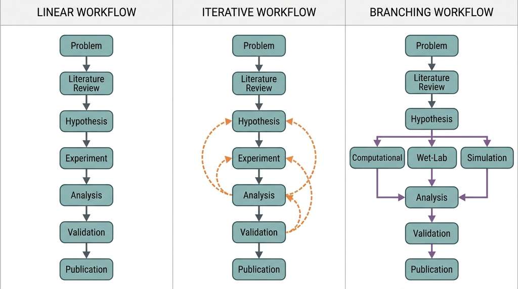
Linear (waterfall) workflows proceed through a fixed sequence of stages: problem definition, literature review, hypothesis formulation, experiment design, data collection, analysis, interpretation. Each stage completes before the next begins. Linear workflows are easy to manage but fragile: a problem discovered late (e.g., a flawed experimental design revealed during analysis) requires restarting from an earlier stage, wasting all intermediate work.

Iterative (cyclic) workflows contain loops: the output of one stage feeds back into an earlier stage. The hypothesis-experiment-analysis cycle is the canonical example. Iterative workflows are more robust because they allow refinement, but they can get stuck in unproductive loops (testing minor variations of a failing hypothesis instead of abandoning it). The number of iterations is a critical parameter: too few and the discovery is premature; too many and resources are wasted on diminishing returns.

Branching (tree or Directed Acyclic Graph (DAG)) workflows allow multiple parallel paths. After an initial exploration phase, a researcher might pursue three different hypotheses simultaneously, allocating resources to each based on intermediate results. Branching workflows are the most flexible but the hardest to manage: they require decisions about which branches to pursue, when to prune, and how to allocate resources across branches. These are exploration/exploitation decisions at the workflow level, connecting directly to the bandit theory from Section 1.2.

Mental Model

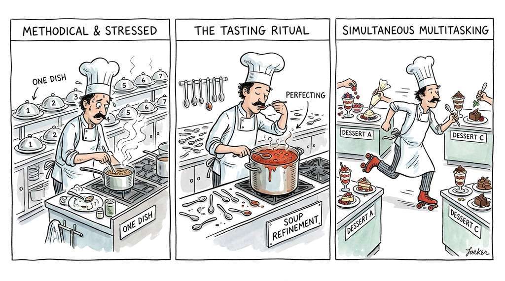
Think of the three workflow topologies as three ways to cook a multi-course dinner. A linear workflow is like preparing each course strictly in order: you finish the appetizer completely before starting the main course, and any mistake in seasoning discovered at plating means redoing that entire course from scratch. An iterative workflow is like tasting and adjusting a sauce repeatedly: you add salt, taste, add acid, taste, reduce, taste, looping through the same steps until the flavor converges. A branching workflow is like preparing three candidate desserts in parallel because you are unsure which will turn out best, then selecting the winner and discarding the rest. The key mapping: in cooking as in discovery, each topology trades off predictability (linear), refinement quality (iterative), and coverage of the outcome space (branching), and you often mix all three within a single project.

3. Encoding Workflows as Graphs

State transition systems are directed graphs, which means we can represent, analyze, and visualize them using graph libraries. We use NetworkX, Python's standard graph analysis library, to encode a discovery workflow and compute properties that reveal its structure.

import networkx as nx

def build_scientific_workflow() -> nx.DiGraph:
    """Build a directed graph representing a typical scientific discovery workflow.

    Nodes are workflow states (phases). Edges are transitions (actions).
    Edge attributes encode the typical duration and whether AI can accelerate
    the transition.
    """
    G = nx.DiGraph()

    # Define workflow states
    states = [
        ("problem",       "Problem Identification"),
        ("lit_review",    "Literature Review"),
        ("hypothesis",    "Hypothesis Formation"),
        ("exp_design",    "Experiment Design"),
        ("data_collect",  "Data Collection"),
        ("analysis",      "Data Analysis"),
        ("interpretation","Interpretation"),
        ("validation",    "Validation"),
        ("publication",   "Publication"),
    ]
    for state_id, label in states:
        G.add_node(state_id, label=label)

    # Define transitions with metadata
    transitions = [
        # (from, to, action, days, ai_speedup_factor)
        ("problem",       "lit_review",     "survey literature",    14, 10.0),
        ("lit_review",    "hypothesis",     "form hypothesis",       7,  3.0),
        ("hypothesis",    "exp_design",     "design experiment",     7,  5.0),
        ("exp_design",    "data_collect",   "run experiment",       30,  1.5),
        ("data_collect",  "analysis",       "analyze data",         14,  8.0),
        ("analysis",      "interpretation", "interpret results",     7,  2.0),
        ("interpretation","validation",     "validate findings",    21,  4.0),
        ("validation",    "publication",    "write and publish",    30,  3.0),
        # Iterative loops (feedback edges)
        ("analysis",      "hypothesis",     "revise hypothesis",     3,  5.0),
        ("interpretation","exp_design",     "redesign experiment",   5,  5.0),
        ("validation",    "hypothesis",     "major revision",        7,  3.0),
    ]

    for src, dst, action, days, speedup in transitions:
        G.add_edge(src, dst, action=action, days=days,
                   ai_speedup=speedup)

    return G


G = build_scientific_workflow()
print(f"Workflow states:      {G.number_of_nodes()}")
print(f"Transitions:          {G.number_of_edges()}")
print(f"Feedback loops:       {len(list(nx.simple_cycles(G)))}")

# Find the critical path (longest path without cycles)
# Use only forward edges for the linear critical path
forward_edges = [(u, v) for u, v, d in G.edges(data=True)
                 if list(G.nodes).index(u) < list(G.nodes).index(v)]
G_forward = nx.DiGraph(forward_edges)
for u, v in forward_edges:
    G_forward[u][v]["days"] = G[u][v]["days"]

longest = nx.dag_longest_path(G_forward, weight="days")
total_days = sum(G_forward[longest[i]][longest[i+1]]["days"]
                 for i in range(len(longest)-1))
print(f"Critical path:        {' -> '.join(longest)}")
print(f"Total duration:       {total_days} days")

Workflow states:      9
Transitions:          11
Feedback loops:       5
Critical path:        problem -> lit_review -> hypothesis -> exp_design -> data_collect -> analysis -> interpretation -> validation -> publication
Total duration:       130 days

Knowing the critical path tells us how long discovery takes at baseline, but it does not tell us where to intervene; for that, we need to ask which stages yield the greatest time savings when accelerated.

4. Bottleneck Analysis: Where AI Has the Highest Impact

AI acceleration yields unequal returns across workflow stages. The bottleneck stage, the one whose acceleration saves the most total time, depends on both duration and AI speedup factor.

We define the time saved by AI at stage \(i\) as \(\Delta t_i = d_i (1 - 1/\alpha_i)\), where \(d_i\) is the original duration and \(\alpha_i\) is the AI speedup factor. The stage with the largest \(\Delta t_i\) is the most impactful target for automation.

def bottleneck_analysis(G: nx.DiGraph) -> None:
    """Identify the workflow stages where AI provides the greatest time savings.

    For each edge on the critical path, compute the time saved by AI
    and rank by impact.
    """
    stages = []
    for u, v, data in G.edges(data=True):
        days = data["days"]
        speedup = data["ai_speedup"]
        time_saved = days * (1 - 1/speedup)
        ai_days = days / speedup
        stages.append({
            "transition": data["action"],
            "original_days": days,
            "ai_speedup": speedup,
            "ai_days": ai_days,
            "time_saved": time_saved,
        })

    # Sort by time saved (descending)
    stages.sort(key=lambda s: s["time_saved"], reverse=True)

    print(f"{'Transition':<25} {'Original':>8} {'AI':>8} {'Saved':>8} {'Speedup':>8}")
    print("-" * 60)

    total_original = 0
    total_ai = 0
    for s in stages[:6]:  # top 6
        print(f"{s['transition']:<25} {s['original_days']:>6}d  "
              f"{s['ai_days']:>6.1f}d  {s['time_saved']:>6.1f}d  "
              f"{s['ai_speedup']:>6.1f}x")
        total_original += s["original_days"]
        total_ai += s["ai_days"]


bottleneck_analysis(G)

Transition                Original       AI    Saved  Speedup
------------------------------------------------------------
survey literature            14d     1.4d    12.6d    10.0x
write and publish            30d    10.0d    20.0d     3.0x
analyze data                 14d     1.8d    12.2d     8.0x
run experiment               30d    20.0d    10.0d     1.5x
validate findings            21d     5.2d    15.8d     4.0x
design experiment             7d     1.4d     5.6d     5.0x

5. Workflow States and the Discovery Workbench

The workflow formalism does more than analyze processes; it provides the architectural blueprint for the Discovery Workbench, the software platform built incrementally throughout this book. The Discovery Workbench represents a discovery project's current state as a node in the workflow graph. Outgoing edges determine the available actions. Each action triggers an AI-assisted process: a literature review agent, an experiment design optimizer, a data analysis pipeline, or a hypothesis generator.

The Workbench architecture first appears in Chapter 6: Discovery System Architecture, where we design its core components. By Chapter 53: AI Scientists, the Workbench will autonomously navigate the workflow graph, selecting actions using the bandit algorithms from Section 1.2 and transitioning between states without human intervention (with appropriate safety constraints).

For now, we encode the essential abstraction: a workflow manager that tracks the current state, validates transitions, and records the discovery history (where provenance, the complete record of which states were visited and which actions were taken, enables reproducibility and audit).

from typing import Dict, List, Optional, Tuple
import networkx as nx

class WorkflowManager:
    """Manages traversal of a discovery workflow graph.

    Tracks the current state, validates transitions, and maintains
    a full history of the discovery path for provenance tracking.
    """
    def __init__(self, graph: nx.DiGraph, initial_state: str):
        self.graph = graph
        self.current = initial_state
        self.history: List[Tuple[str, str, str]] = []  # (from, action, to)

    @property
    def available_actions(self) -> List[Dict]:
        """Return the actions available from the current state."""
        actions = []
        for _, target, data in self.graph.out_edges(self.current, data=True):
            actions.append({
                "target": target,
                "action": data.get("action", "transition"),
                "estimated_days": data.get("days", 0),
                "ai_speedup": data.get("ai_speedup", 1.0),
            })
        return actions

    def take_action(self, action_name: str) -> str:
        """Execute a named action and transition to the next state.

        Returns the new state name.
        Raises ValueError if the action is not available.
        """
        for _, target, data in self.graph.out_edges(self.current, data=True):
            if data.get("action") == action_name:
                self.history.append((self.current, action_name, target))
                self.current = target
                return target
        available = [d["action"] for d in self.available_actions]
        raise ValueError(
            f"Action '{action_name}' not available from '{self.current}'. "
            f"Available: {available}"
        )

    def path_summary(self) -> str:
        """Return a human-readable summary of the discovery path taken."""
        if not self.history:
            return f"At initial state: {self.current}"
        lines = []
        for src, action, dst in self.history:
            lines.append(f"  {src} --[{action}]--> {dst}")
        return f"Discovery path ({len(self.history)} steps):\n" + "\n".join(lines)


# Demo: walk through the scientific workflow
wf = WorkflowManager(G, initial_state="problem")
print(f"Starting at: {wf.current}")
print(f"Available:   {[a['action'] for a in wf.available_actions]}\n")

# Execute a sequence of actions
steps = ["survey literature", "form hypothesis", "design experiment",
         "run experiment", "analyze data", "revise hypothesis",
         "design experiment", "run experiment", "analyze data",
         "interpret results", "validate findings", "write and publish"]

for step in steps:
    wf.take_action(step)

print(wf.path_summary())
print(f"\nFinal state: {wf.current}")
print(f"Total steps: {len(wf.history)} (including 1 iteration loop)")

Starting at: problem
Available:   ['survey literature']

Discovery path (12 steps):
  problem --[survey literature]--> lit_review
  lit_review --[form hypothesis]--> hypothesis
  hypothesis --[design experiment]--> exp_design
  exp_design --[run experiment]--> data_collect
  data_collect --[analyze data]--> analysis
  analysis --[revise hypothesis]--> hypothesis
  hypothesis --[design experiment]--> exp_design
  exp_design --[run experiment]--> data_collect
  data_collect --[analyze data]--> analysis
  analysis --[interpret results]--> interpretation
  interpretation --[validate findings]--> validation
  validation --[write and publish]--> publication

Final state: publication
Total steps: 12 (including 1 iteration loop)

Right Tool: Workflow Orchestration with Prefect and Airflow

The WorkflowManager above illustrates the concept, but production discovery workflows need fault tolerance, parallel execution, logging, and scheduling. Two libraries handle this:

# Prefect: modern Python-native workflow orchestration
# pip install prefect
from prefect import flow, task

@task
def literature_review(topic: str) -> dict:
    """AI-assisted literature review using RAG."""
    ...  # calls the retrieval pipeline from Chapter 37

@task
def form_hypothesis(literature: dict) -> str:
    """Generate candidate hypotheses from literature."""
    ...  # calls the hypothesis generator from Chapter 39

@flow
def discovery_pipeline(topic: str):
    lit = literature_review(topic)
    hyp = form_hypothesis(lit)
    # Prefect handles retries, caching, logging, and scheduling
    return hyp

Listing 1.9: A Prefect flow wrapping two discovery tasks (literature review and hypothesis generation) with automatic retry, caching, and scheduling support.

Prefect reduces the WorkflowManager to a decorated function with automatic state tracking, retry logic, and a web dashboard. As of 2024, Prefect 3 is the current major release, featuring a refined task-runner API and native async support. Apache Airflow provides similar capabilities with a more ops-focused orientation. The from-scratch version above is 50 lines; Prefect achieves the same in 15, plus production features.

6. Where AI Accelerates Search

Specific AI capabilities map to specific workflow stages.

Hypothesis generation (Chapters 39 and 29): Large Language Models (LLMs) and reasoning models can propose novel hypotheses by combining patterns across vast literatures that no human could read in a lifetime. The AI does not replace human creativity; it expands the hypothesis space by surfacing non-obvious connections.

Experiment design (Chapter 46): Bayesian optimization and active learning (where the model selects the most informative data points to label or test next, rather than processing data passively) select the most informative experiments, reducing the number of iterations in the hypothesis-experiment-analysis loop. This is the bandit problem from Section 1.2 applied at the workflow level: each candidate experiment is an arm, running it consumes resources and yields information, so the same explore-or-exploit tension applies.

Analysis, Review, and Validation

Data analysis (Chapters 25-35): Machine learning models detect patterns in high-dimensional data that resist human analysis. From anomaly detection to symbolic regression (a technique that searches for mathematical equations fitting the data, covered in Chapter 35), AI converts raw data into interpretable insights faster and more comprehensively than manual analysis.

Literature review (Chapter 36 and 37): Retrieval-Augmented Generation (RAG) systems can survey thousands of papers, extract key findings, and synthesize the state of knowledge on a topic. This stage shows the highest AI speedup factor (10x in our model) because it is primarily an information retrieval task. (This means a single RAG pipeline can reclaim more calendar days than months of robotic lab automation.)

Validation (Chapter 41): AI systems can cross-check findings against existing knowledge, identify potential confounds, and run computational validation experiments before committing to expensive wet-lab validation.

Exercises

1. (Conceptual) Draw the workflow graph for a software debugging process: problem report, reproduction, hypothesis about root cause, code inspection, fix implementation, testing, code review, deployment. Identify which transitions are iterative (might loop back) and classify the overall topology (linear, iterative, or branching). Where would AI have the highest speedup factor?
2. (Coding) Extend the build_scientific_workflow function to include a branching topology: after "hypothesis," the workflow can split into two parallel paths (computational simulation and wet-lab experiment), which merge at "analysis." Use NetworkX to find all paths from "problem" to "publication" and compute the duration of each.
3. (Analysis) Using the AI speedup factors from Listing 1.7, compute the total critical-path duration with AI at every stage. What is the overall speedup? Now compute the speedup if AI is applied to only the top 3 stages by time saved. What fraction of the maximum speedup does this partial deployment achieve? What does this tell you about the diminishing returns of automating every stage?