Prerequisites
This section opens the chapter on Bayesian discovery. You should be comfortable with probability distributions and Bayes' theorem from Appendix A, and with the general concept of statistical models from Chapter 5. We build on the data exploration skills from Chapter 25. No prior experience with PyMC or probabilistic programming is assumed; we start from first principles.
A Bayesian model is not just a curve-fitting tool. It is a formal encoding of a scientific hypothesis: "I believe the world works this way, with these unknowns, and this is how observations connect to those unknowns." The Bayesian workflow makes this encoding explicit, testable, and improvable. You start with a prior (what you believe before data), define a likelihood (how data arises given your hypothesis), compute a posterior (what you believe after data), and then check whether the model is any good through predictive checks. When the model fails, you diagnose why, revise, and iterate. This section teaches you to build, check, and refine Bayesian models as a disciplined scientific practice.
1. Bayesian Models as Scientific Hypotheses
In 2015, physicists at LIGO faced a question no amount of raw data could answer on its own: given a faint ripple in a detector's signal, what was the probability that two black holes had just merged a billion light-years away, versus the probability that the instrument had glitched? The framework that let them assign a credible answer, and quantify exactly how uncertain that answer remained, is the same one you will build in this section.
When a clinical trial estimates a drug's effect without quantifying uncertainty, regulators cannot distinguish a genuine benefit from statistical noise, and patients bear the consequences of that ambiguity. The Bayesian workflow exists to make uncertainty explicit and actionable, turning vague confidence into calibrated probability statements that support real decisions.
Every Bayesian model consists of three components. The prior \(p(\theta)\) encodes what you know (or assume) about the parameters \(\theta\) before seeing data. The likelihood \(p(D \mid \theta)\) describes the probability of observing data \(D\) given parameter values. And the posterior \(p(\theta \mid D)\) is what you learn from combining the two through Bayes' theorem:
The posterior is a complete probability distribution over parameter values, conditioned on observed data. It tells you not just the best estimate of each parameter but the full range of plausible values and their relative credibilities. Point estimates alone can mislead when data are noisy or scarce; the posterior width directly quantifies how much the data constrain your hypothesis. The mechanism is multiplicative: at each candidate parameter value, you multiply the prior probability by the likelihood of the observed data under that value. The normalized product gives the posterior weight. Use posterior inference when you need calibrated uncertainty bands, want to incorporate prior knowledge from earlier experiments, or plan to compare competing models on the same data. Prefer maximum likelihood when the dataset is large enough that the prior's contribution is negligible and you need only a point prediction.
The Posterior in One Equation
$$p(\theta \mid D) = \frac{p(D \mid \theta) \, p(\theta)}{p(D)}$$The denominator \(p(D) = \int p(D \mid \theta) \, p(\theta) \, d\theta\) is the marginal likelihood (or evidence), a normalizing constant that ensures the posterior integrates to one. Computing this integral is the central computational challenge of Bayesian inference, and it is what motivates the Markov chain Monte Carlo (MCMC) and variational methods we cover in Section 32.2. In short: the posterior is just a weighted compromise between what you believed before (the prior) and what the data tell you (the likelihood), and every computational method in this chapter exists to evaluate that compromise efficiently.
Mental Model
Think of the posterior like updating a weather forecast. Before checking any instruments, a forecaster has a prior belief about tomorrow's temperature based on the season and recent trends (the prior). Each new reading, a barometer, a satellite image, a wind measurement, adjusts that belief proportionally to how reliable the instrument is (the likelihood). After processing all the readings, the forecaster's updated prediction is not a single number but a range: "75 to 82 degrees, most likely around 78" (the posterior distribution). Just as a forecaster who ignores all instruments is guessing, and one who ignores seasonal context is naive, a Bayesian model combines both sources of information, weighting each by its informativeness. The marginal likelihood corresponds to how well the forecasting model as a whole predicted the readings it actually received: models that assigned high probability to the observed data score well, regardless of which specific temperature they favored.
This framework turns competing scientific hypotheses into competing models. If a chemical reaction rate varies with temperature, one hypothesis posits an Arrhenius relationship (an exponential dependence on inverse temperature, derived from activation energy theory) while another posits a power law; each defines its own likelihood function. You can fit both to the same data, compare them quantitatively (Section 32.3), and determine which the data support more strongly.
Frequentist critics often object to the subjectivity of priors. But in scientific applications, the prior is precisely where domain knowledge enters the model. A chemist who knows that reaction rate constants are positive is encoding real information. A physicist who knows that a mass cannot be negative is ruling out physically impossible parameter values. Far from being a weakness, the prior is the mechanism by which Bayesian models incorporate the accumulated knowledge of a scientific field. The key discipline is making the prior explicit, checking its implications, and being transparent about what it rules in and out.
2. Choosing Priors
Prior selection is the most contested part of Bayesian analysis, and for good reason: the prior directly affects the posterior, especially when data are scarce. Three broad strategies cover most scientific applications.
Uninformative (Flat) Priors
A flat prior \(p(\theta) \propto 1\) says "all parameter values are equally plausible." This sounds objective, but it is not. On the real line, a flat prior is improper (it does not integrate to a finite value), which can cause computational problems. On a bounded interval, a uniform prior is proper but still embeds assumptions: a uniform prior on a rate constant \(k \in [0, 100]\) implies that \(k = 99\) is just as plausible as \(k = 0.01\), which no chemist would endorse. Flat priors are useful as baselines but rarely represent genuine scientific indifference.
Common Misconception
A common misconception is that "uninformative" priors are objective or assumption-free. In reality, every prior encodes assumptions: a flat prior on a parameter is not flat after a nonlinear transformation (for example, a uniform prior on a rate constant \(k\) implies a non-uniform prior on \(\log k\)), and an improper flat prior can silently produce an improper posterior that no sampling algorithm can rescue. No prior is truly "without assumptions"; the honest practice is to choose a prior whose assumptions you can defend and then verify through prior predictive checks that those assumptions produce sensible simulated data.
Weakly Informative Priors
The recommendation from Gelman et al. (2020) is to use weakly informative priors that rule out clearly implausible values without strongly favoring any particular region. For a parameter you expect to be "around 1, give or take an order of magnitude," a \(\text{Normal}(0, 10)\) or \(\text{HalfNormal}(10)\) prior on the appropriate scale (log, logit (the log-odds transform, used for parameters bounded between 0 and 1), etc.) is weakly informative. The idea is to let the data dominate in regions where you have observations, while preventing the sampler from exploring physically meaningless territory.
Domain-Informed Priors
For discovery applications, the most valuable priors are those that encode genuine domain knowledge. If previous experiments measured a binding affinity of \(K_d = 50 \pm 15\) nM, using \(\text{Normal}(50, 15)\) as a prior for \(K_d\) in a new experiment on a related compound is not subjective bias; it is efficient use of accumulated scientific knowledge. The posterior from one experiment becomes the prior for the next, making Bayesian updating a natural model for the scientific literature.
Let us build a concrete example. A materials scientist is studying how the yield strength \(\sigma_y\) of an alloy depends on grain size \(d\). The Hall-Petch relationship predicts \(\sigma_y = \sigma_0 + k_{\text{HP}} \, d^{-1/2}\). We encode this as a Bayesian model in PyMC, a Python library for specifying and fitting probabilistic models using automatic posterior sampling:
import pymc as pm
import numpy as np
import arviz as az

# Simulated grain-size data (micrometers) and yield strength (MPa)
rng = np.random.default_rng(42)
d_obs = rng.uniform(5, 100, size=30)           # grain sizes
sigma_0_true, k_hp_true = 50.0, 500.0          # true parameters
sigma_y_obs = sigma_0_true + k_hp_true * d_obs**(-0.5) + rng.normal(0, 8, size=30)

with pm.Model() as hall_petch_model:
    # Weakly informative priors grounded in physical knowledge
    sigma_0 = pm.Normal("sigma_0", mu=0, sigma=100)     # friction stress (MPa)
    k_hp = pm.HalfNormal("k_hp", sigma=1000)            # Hall-Petch slope (positive)
    noise = pm.HalfNormal("noise", sigma=20)             # measurement noise

    # Deterministic Hall-Petch relationship
    mu = sigma_0 + k_hp * d_obs**(-0.5)

    # Likelihood: observed yield strengths
    y_obs = pm.Normal("y_obs", mu=mu, sigma=noise, observed=sigma_y_obs)

print(hall_petch_model)
k_hp encodes the physical constraint that the Hall-Petch slope must be positive. The noise parameter captures measurement uncertainty.
The Hall-Petch slope \(k_{\text{HP}}\) is physically constrained to be non-negative:
finer grains always strengthen (or at least do not weaken) the material, up to the
inverse Hall-Petch regime at nanometer scales. Using pm.HalfNormal
enforces this constraint automatically. If we had used pm.Normal, the
sampler would waste time exploring negative values, and the posterior might place
some mass in physically impossible territory. Domain constraints like this are one
of the strongest advantages of the Bayesian approach: you cannot express "this
parameter must be positive" in an ordinary least-squares fit without adding an
explicit constraint optimizer, but in a Bayesian model it is simply the choice of
prior distribution.
3. Likelihoods for Common Scientific Data
With priors encoding what we believe before seeing data, the next question is how to formalize the connection between those beliefs and the measurements we actually collect.
The likelihood function connects your model's parameters to the data you actually observe. Choosing the right likelihood is as important as choosing the right prior, and the choice depends on the data-generating process. Table 32.1 summarizes the most common likelihood functions for scientific data types.
| Data Type | Distribution | PyMC Syntax | When to Use |
|---|---|---|---|
| Continuous, symmetric errors | Normal | pm.Normal("y", mu=..., sigma=...) | Most regression problems with Gaussian noise |
| Continuous, heavy-tailed errors | Student-t | pm.StudentT("y", nu=..., mu=..., sigma=...) | Outlier-robust regression; spectroscopic data |
| Count data | Poisson | pm.Poisson("y", mu=...) | Photon counts, mutation counts, event rates |
| Count data with overdispersion | Negative Binomial | pm.NegativeBinomial("y", mu=..., alpha=...) | RNA-seq, ecological counts with variance > mean |
| Binary outcomes | Bernoulli | pm.Bernoulli("y", p=...) | Success/failure experiments, classification |
| Proportions | Beta | pm.Beta("y", alpha=..., beta=...) | Fractions, concentrations bounded in [0,1] |
| Positive continuous | Lognormal / Gamma | pm.LogNormal("y", mu=..., sigma=...) | Concentrations, lifetimes, particle sizes |
A frequent mistake is defaulting to a Normal likelihood for all continuous data. If your measurements are strictly positive (concentrations, intensities, durations), a Lognormal or Gamma likelihood respects that constraint and often fits better. If your data have occasional large outliers (common in spectroscopy or environmental monitoring), a Student-t likelihood with low degrees of freedom \(\nu\) provides robustness that a Normal likelihood cannot. The choice of likelihood is itself a scientific hypothesis about how noise enters your measurement process.
4. Prior Predictive Checks
Before fitting the model to real data, we should check whether the prior produces reasonable data. A prior predictive check samples parameters from the prior, generates synthetic data, and asks: "Does this look anything like data I might actually observe?" If your prior predictive distribution includes yield strengths of \(-10{,}000\) MPa or \(+10^{12}\) MPa, the prior is too vague. If it concentrates all mass within \(\pm 1\) MPa of a particular value, it is too informative and will overwhelm the data.
with hall_petch_model:
    prior_pred = pm.sample_prior_predictive(samples=500, random_seed=42)

# Inspect the prior predictive distribution
prior_y = az.extract(prior_pred.prior_predictive)["y_obs"].values
print(f"Prior predictive range: [{prior_y.min():.0f}, {prior_y.max():.0f}] MPa")
print(f"Prior predictive mean:  {prior_y.mean():.0f} MPa")
print(f"Prior predictive std:   {prior_y.std():.0f} MPa")

# Visualize with ArviZ
az.plot_ppc(prior_pred, group="prior", num_pp_samples=100)
sample_prior_predictive. ArviZ's plot_ppc overlays 100 simulated datasets drawn from the prior against the observed data, revealing whether the prior range is physically plausible.
The prior predictive check is the Bayesian analogue of a unit test. It catches
modeling errors before you spend computational resources on inference. Gelman et al.
(2020) recommend it as the first step in every Bayesian analysis, and modern tools
make it nearly free: sample_prior_predictive requires no MCMC and runs
in seconds. (A full MCMC posterior takes minutes to hours; a prior predictive check takes under one second on the same model, yet it catches the majority of specification errors before you spend any of that compute.)
The prior predictive visualization above uses az.plot_ppc, which handles
all the formatting: overlay of simulated data draws, comparison with observed data,
kernel density estimation (KDE), and proper labeling. Without ArviZ, a companion library to PyMC that provides diagnostic plots and summary statistics for Bayesian models, you would need roughly
40 lines of Matplotlib code to produce the same plot. ArviZ also provides
az.plot_prior for visualizing the prior distributions themselves, and
az.summary for tabular summaries with HDI intervals. In practice, the library
can reduce diagnostic code by roughly an order of magnitude compared to manual plotting.
5. The Iterative Model-Building Cycle
The Bayesian workflow is not "specify model, press run, report results." It is an iterative cycle of model building, checking, and revision. Gelman et al. (2020) describe this cycle explicitly. Figure 32.1 illustrates the six steps and the feedback loop that drives model improvement. Figure 32.1.1 illustrates the iterative Bayesian model-building cycle.
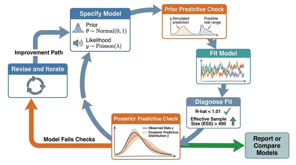
- Specify the model. Choose priors and likelihood based on domain knowledge and the data-generating process.
- Prior predictive check. Simulate data from the prior; verify that it covers the plausible range without extending into nonsense.
- Fit the model. Run MCMC or variational inference (VI) to approximate the posterior (covered in Section 32.2).
- Diagnose the fit. Check convergence (R-hat, a statistic that compares within-chain and between-chain variance to detect non-convergence, effective sample size (ESS), divergences, where a divergence is a numerical failure in the sampler that signals the posterior geometry is too difficult for the current configuration) to ensure the posterior samples are trustworthy.
- Posterior predictive check. Simulate data from the fitted model; compare to the observed data. Systematic mismatches reveal model misspecification.
- Revise and iterate. If the model fails checks, diagnose why (wrong likelihood? missing covariate? prior too tight?) and return to step 1.
Checkpoint
So far: a Bayesian model encodes a scientific hypothesis through three components (prior, likelihood, posterior), and the six-step iterative cycle ensures that each model is checked against simulated and observed data before its conclusions are trusted.
Let us complete the cycle for our Hall-Petch model by running the fit and performing posterior predictive checks:
with hall_petch_model:
    # Step 3: Fit the model with NUTS (default in PyMC)
    trace = pm.sample(2000, tune=1000, chains=4, random_seed=42)

    # Step 4: Diagnose convergence
    summary = az.summary(trace, var_names=["sigma_0", "k_hp", "noise"])
    print(summary[["mean", "sd", "hdi_3%", "hdi_97%", "r_hat", "ess_bulk"]])

    # Step 5: Posterior predictive check
    post_pred = pm.sample_posterior_predictive(trace, random_seed=42)

# Visualize the posterior predictive check
az.plot_ppc(post_pred, num_pp_samples=100)
az.summary call reports R-hat (should be < 1.01), ESS (should be > 400), and HDI (highest density interval), the narrowest interval containing a specified probability mass. The posterior predictive check overlays simulated data from the fitted model against the observations.The posterior predictive check is widely regarded as one of the most powerful diagnostics in the Bayesian toolkit. If the model is well-specified, data simulated from the posterior should be statistically indistinguishable from the observed data. Systematic deviations (for example, the model consistently underestimates yield strength at very small grain sizes) point to specific model failures and suggest specific fixes (in this case, adding an inverse Hall-Petch correction term for nanoscale grains).
The classical Bayesian workflow requires running a fresh MCMC chain for every new dataset, which becomes a bottleneck when thousands of datasets must be analyzed (as in gravitational-wave astronomy or particle physics). Radev et al. (2023) introduced BayesFlow, a framework for amortized Bayesian inference: a neural network is trained once on simulated data from the generative model and then produces approximate posteriors for any new observation in milliseconds, without additional sampling. The BayesFlow paper ("BayesFlow: Amortized Bayesian Workflows With Neural Networks," Journal of Open Source Software, 8(89), 5702) demonstrates that this approach preserves calibration (validated via simulation-based calibration from Talts et al., 2018) while accelerating inference by orders of magnitude. This amortized approach is especially promising for the iterative model-building cycle described above: rapid posterior feedback lets the scientist revise priors and likelihoods interactively rather than waiting hours for each MCMC run. As of 2024, BayesFlow 2.0 introduced a redesigned modular API with composable inference and summary networks, broadening its applicability beyond the original architecture; practitioners starting new projects should consult the BayesFlow 2.0 documentation for the current interface.
6. From Single Models to Model Comparison
The workflow described above applies to a single model. But scientific discovery often involves comparing competing hypotheses, not just fitting one. Does the data favor an Arrhenius model or a power-law model? Is a linear dose-response adequate, or does a sigmoidal model fit better? The Bayesian framework handles model comparison naturally through the marginal likelihood, leave-one-out cross-validation (LOO-CV), and the widely applicable information criterion (WAIC), which we develop in Section 32.3.
Model comparison in the Bayesian framework is not about finding the model that "fits best" in the sense of minimizing residuals. A model with enough parameters can fit any dataset perfectly, but that does not make it scientifically useful. Bayesian model comparison penalizes complexity through the marginal likelihood. A simpler model that explains the data almost as well as a complex one scores a higher marginal likelihood, because its prior concentrates more mass on the parameter values that actually generated the data. This built-in Occam's razor (the principle that simpler explanations should be preferred when they account for the data equally well) is one of the strongest arguments for the Bayesian approach in scientific discovery.
There is a deep analogy between Bayesian updating and the way scientific communities actually work. A researcher publishes a finding with a confidence interval. Other researchers treat that finding as prior information for their own experiments. Over time, the community's collective belief tends to converge toward well-supported conclusions (or at least toward a posterior with progressively narrower uncertainty). The Bayesian framework formalizes what scientists already do informally: start with beliefs, update them with evidence, and report what remains uncertain. The difference is that the Bayesian version is explicit, reproducible, and auditable.
7. When Not to Use Bayesian Methods
Model comparison gives the Bayesian framework its scientific teeth, but that power comes with real costs in computation and modeling effort that make it the wrong choice in some situations.
Bayesian methods are not always the right tool. They are computationally expensive compared to frequentist alternatives (though this gap is shrinking). They require explicit model specification, which can be difficult for complex systems where the data-generating process is poorly understood. And they can give misleading results when the model is misspecified and the analyst does not perform posterior predictive checks.
Concrete cases where frequentist or machine learning approaches may be preferable:
- Pure prediction with no need for uncertainty. If you only need a point prediction and do not care about confidence intervals, gradient-boosted trees or neural networks are faster and often more accurate. See Chapter 26.
- Very large datasets with simple models. When \(n > 10^6\) and the model is a standard regression, the posterior is essentially determined by the data, and the prior is irrelevant. Maximum likelihood gives the same answer much faster.
- Exploratory analysis before model specification. The exploratory discovery techniques of Chapter 25 are better for initial data understanding. Bayesian modeling comes after you have a hypothesis to test.
The Bayesian workflow shines when uncertainty quantification matters, when you have genuine prior information, when you need to compare competing hypotheses, and when the dataset is small enough that the prior has real influence. These conditions describe a large fraction of scientific research.
Try It: Prior Sensitivity Dashboard
Build a small experiment that visualizes how prior choice affects the posterior, using only PyMC, ArviZ, and Matplotlib.
- Generate a synthetic dataset of 20 observations from a known Normal distribution
with mean 5.0 and standard deviation 2.0 using
numpy.random.default_rng(0).normal(5.0, 2.0, 20). - Define a PyMC model with a Normal likelihood and a Normal prior on the mean parameter. Create four variants of the model by setting the prior standard deviation to 0.5, 2, 10, and 100 (keeping the prior mean at 0 for all four).
- For each variant, run
pm.sample_prior_predictive(500)andpm.sample(1000, tune=500, chains=2), then collect the posterior samples for the mean parameter. - Plot a 2x2 grid of panels (one per prior width) showing the prior density, the
likelihood profile, and the resulting posterior density overlaid. Use
az.plot_posterioror manual KDE plots withscipy.stats.gaussian_kde. - Add a text annotation to each panel showing the posterior mean and 94% HDI width. Observe how the posterior shifts from prior-dominated (narrow prior, wide HDI relative to prior) to data-dominated (wide prior, HDI converges to the sample mean) as the prior standard deviation increases.
Exercise 32.1.1
A researcher models enzyme activity \(v\) as a function of substrate concentration \([S]\)
using the Michaelis-Menten equation: \(v = V_{\max} [S] / (K_m + [S])\). She places a
Normal(0, 1000) prior on \(V_{\max}\) and a Normal(0, 1000)
prior on \(K_m\). Run a prior predictive check by sampling 500 draws from these priors,
computing \(v\) at \([S] = 1.0\), and plotting the distribution. What fraction of prior
draws produce negative \(v\) values, and why is this a problem? Propose a better pair of
priors that respects the physical constraints (\(V_{\max} > 0\), \(K_m > 0\)) and re-run
the prior predictive check to confirm improvement.
Hint
Both \(V_{\max}\) and \(K_m\) are strictly positive physical quantities. Replace each
Normal prior with a HalfNormal or LogNormal
prior. After the swap, the prior predictive distribution of \(v\) should contain no
negative values. You can compute the fraction of negative draws with
(v_samples < 0).mean().
Step-Through: One Round of Bayesian Updating
Trace through Bayes' theorem with a tiny discrete example. Suppose a coin has an unknown bias \(\theta\) and we consider only three candidate values: \(\theta \in \{0.3, 0.5, 0.7\}\).
Prior: We start with equal belief: \(p(\theta=0.3) = p(\theta=0.5) = p(\theta=0.7) = 1/3 \approx 0.333\).
Observation: We flip the coin once and observe Heads (\(D = H\)).
Likelihoods: \(p(H \mid 0.3) = 0.3\), \(\; p(H \mid 0.5) = 0.5\), \(\; p(H \mid 0.7) = 0.7\).
Unnormalized posterior: Multiply prior by likelihood for each value: \(0.333 \times 0.3 = 0.100\), \(\; 0.333 \times 0.5 = 0.167\), \(\; 0.333 \times 0.7 = 0.233\).
Marginal likelihood: \(p(D) = 0.100 + 0.167 + 0.233 = 0.500\).
Normalized posterior: \(p(0.3 \mid H) = 0.100/0.500 = 0.200\), \(\; p(0.5 \mid H) = 0.167/0.500 = 0.333\), \(\; p(0.7 \mid H) = 0.233/0.500 = 0.467\).
After one Heads observation, belief has shifted toward higher bias values. The posterior on \(\theta = 0.7\) rose from 0.333 to 0.467, while \(\theta = 0.3\) fell from 0.333 to 0.200. This is the multiplicative mechanism at work: candidates that assign higher probability to the observed data gain posterior weight.
Real-World Application: Pharmacokinetics at Novartis
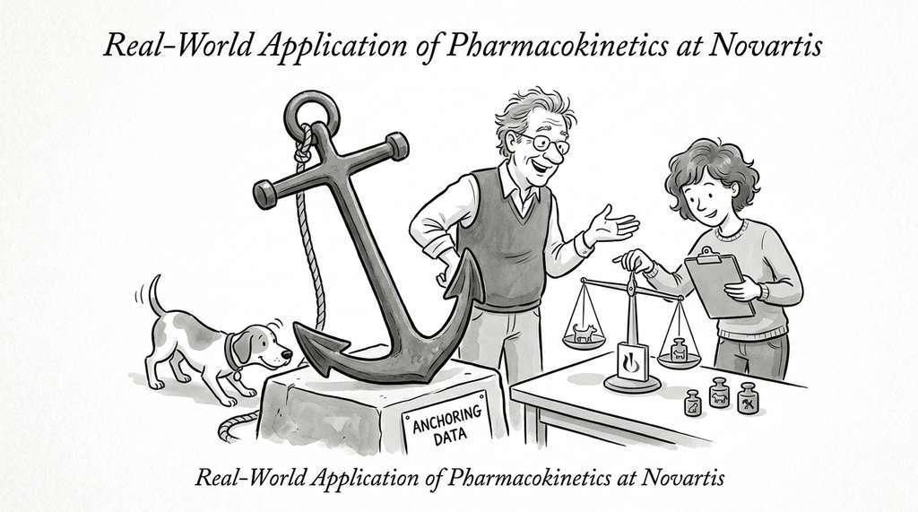
Novartis uses Bayesian population pharmacokinetic (PopPK) models built in Stan and Torsten to estimate drug clearance rates across patient subgroups during clinical trials. Domain-informed priors from preclinical animal studies anchor the clearance and volume-of-distribution parameters, while the likelihood captures inter-patient variability and measurement noise. Prior predictive checks ensure the model does not predict physiologically impossible drug concentrations (for example, negative plasma levels or half-lives shorter than one minute) before any patient data are analyzed.
Lab: Prior Predictive Safari
Goal: Develop intuition for how prior choices shape the space of data your model considers plausible, before any fitting occurs.
Tools: Python 3.10+, PyMC 5.x, ArviZ, Matplotlib (install with
pip install pymc arviz matplotlib).
Setup (5 min): Build a simple linear regression model in PyMC: \(y = \alpha + \beta x + \varepsilon\), with 10 evenly spaced \(x\) values in \([0, 10]\) and \(\varepsilon \sim \text{Normal}(0, \sigma)\).
What to vary (15 min): Create six prior configurations by combining
two prior families for \((\alpha, \beta)\) (Normal vs. Laplace) with three prior
scales (\(\sigma_{\text{prior}} \in \{0.5, 5, 50\}\)). For each configuration, run
pm.sample_prior_predictive(200) and plot the resulting regression lines
(200 lines overlaid on one axis per configuration, arranged in a 2x3 grid).
What to observe (10 min): Note how narrow priors produce nearly parallel lines clustered around zero, wide priors produce "spaghetti" covering enormous \(y\) ranges, and the Laplace prior produces sparser, sharper line bundles than the Normal prior at the same scale. Record the prior predictive \(y\)-range (min to max) for each configuration. Identify the configuration whose prior predictive range best matches a realistic scenario (for example, predicting exam scores from hours studied) and explain why.
Exercises
- (Conceptual) A pharmaceutical researcher sets a prior of \(\text{Normal}(0, 0.1)\) on a drug effect size, arguing that "most drugs have small effects." A colleague objects that this prior is too informative and will bias the posterior toward zero. Under what conditions is the colleague right? Design a simulation to quantify how much the prior influences the posterior as a function of sample size \(n \in \{10, 50, 200, 1000\}\).
- (Coding) Extend the Hall-Petch model to include an inverse Hall-Petch correction term: \(\sigma_y = \sigma_0 + k_{\text{HP}} \, d^{-1/2} - k_{\text{IHP}} \, d^{-1}\), where \(k_{\text{IHP}} \geq 0\). Implement this in PyMC, run prior predictive checks, fit the model, and compare the posterior predictive distributions of the two models. Does the data prefer the extended model?
- (Analysis) Take the Hall-Petch model and systematically vary the prior on \(k_{\text{HP}}\): try \(\text{HalfNormal}(10)\), \(\text{HalfNormal}(100)\), \(\text{HalfNormal}(1000)\), and \(\text{HalfNormal}(10000)\). For each prior, compute the posterior mean, 94% HDI width, and prior predictive range. At what point does the prior stop influencing the posterior? Relate this to the concept of "prior sensitivity analysis" in Bayesian workflow.
What's Next
We have defined the Bayesian model and checked it with prior and posterior predictive simulations. But we skipped over the hardest part: actually computing the posterior. In Section 32.2: Posterior Inference Methods, we dive into the computational engine, covering MCMC (Metropolis-Hastings, Hamiltonian Monte Carlo, and the NUTS sampler), automatic differentiation VI (ADVI), and normalizing flows (flowMC). We will understand why NUTS works so well, when VI is a better choice, and how to diagnose when inference has gone wrong.
Bibliography
The authoritative reference for the iterative Bayesian model-building cycle presented in this section.
The standard graduate reference for Bayesian statistics, with extensive coverage of prior selection and model checking.
The probabilistic programming framework used throughout this section for model specification and sampling.
The diagnostics and visualization library used for prior/posterior predictive checks and convergence assessment.
Introduced simulation-based calibration for validating inference algorithms, now standard practice in probabilistic programming.
The original Hall-Petch paper establishing the grain-size strengthening relationship used as the running example in this section.