2.1 The Scientific Method Revisited

"Everyone says they follow me, but half of them skip straight from observation to publication. I have feelings about this."

The Scientific Method, at a Philosophy of Science Conference

1. The Five Stages as a Computational Pipeline

When NASA's Mars Climate Orbiter burned up in 1999 because one team used metric units and another used imperial, the failure was not in the science but in the pipeline: observation and prediction were never formally connected, so a unit mismatch went undetected until the spacecraft was lost. Making each stage of the scientific method explicit and testable is not academic tidiness; it is the difference between catching errors early and losing a \$327 million mission.

What would it take to hand the scientific method to a machine and let it run, unsupervised, for a week? Every textbook teaches the method as a cycle, but for our purposes it is more useful to think of it as a pipeline with feedback loops. Each stage takes a well-defined input and produces a well-defined output, which means each stage can, in principle, be implemented as a function.

A computational pipeline, in this context, is a sequence of processing stages where the output of one stage becomes the input of the next, much like an assembly line in a factory. This framing turns the philosophical concept of "doing science" into an engineering specification. Each stage has a type signature (what goes in, what comes out), so we can write tests for it, swap implementations, and pinpoint where a system fails. Data flows forward through observe, hypothesize, predict, test, and revise. Feedback edges carry experimental results backward to trigger new observations and revised hypotheses. Reach for this pipeline model whenever you need to automate any part of the discovery process; when your goal is a single, one-off analysis with no iteration, a simpler script without the loop structure will suffice. Figure 2.1.1 illustrates the scientific method as a computational pipeline with feedback loops.

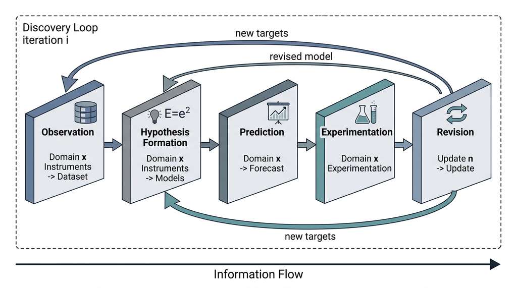
The stages are:

1. Observation: collect data from the world. Input: a domain and instruments. Output: a dataset of measurements.
2. Hypothesis formation: propose an explanation for patterns in the data. Input: observations plus background knowledge. Output: a candidate model or theory.
3. Prediction: derive testable consequences from the hypothesis. Input: a hypothesis. Output: specific, quantitative predictions about unseen data.
4. Experimentation: design and run tests that could distinguish the hypothesis from alternatives. Input: predictions. Output: new observations.
5. Revision: update, refine, or reject the hypothesis in light of experimental results. Input: predictions versus observations. Output: a revised hypothesis or a decision to discard.

The cycle then repeats: revision feeds new observations (because you now know where to look), which feed new hypotheses. Figure 2.1 shows this pipeline with its forward flow and feedback edges. Chapter 1 described discovery as search; the scientific method is the search procedure. The hypothesis space is the search space. Observations are the fitness function. Falsification is the pruning rule.

Let us encode this pipeline in Python, not because we expect to run science through a function call today, but because making the structure explicit reveals where automation is easy, where it is hard, and where it is currently impossible. In short: A hypothesis that cannot be written as a function cannot be tested by a machine, and a method that cannot be written as a loop cannot be automated.

from dataclasses import dataclass, field
from typing import Any, Callable
import numpy as np

@dataclass
class Hypothesis:
    """A scientific hypothesis with a name, a predictive model, and a track record."""
    name: str
    predict: Callable[[np.ndarray], np.ndarray]  # inputs -> predicted outputs
    parameters: dict = field(default_factory=dict)
    falsified: bool = False
    evidence_for: int = 0
    evidence_against: int = 0

    def test(self, inputs: np.ndarray, observed: np.ndarray,
             tolerance: float = 0.05) -> bool:
        """Test the hypothesis against observed data.
        Returns True if predictions match observations within tolerance."""
        predicted = self.predict(inputs)
        residuals = np.abs(predicted - observed)
        matches = np.mean(residuals < tolerance * np.abs(observed).max())
        if matches > 0.95:
            self.evidence_for += 1
            return True
        else:
            self.evidence_against += 1
            return False


def scientific_method(observations, background_knowledge,
                      hypothesis_generator, experiment_designer,
                      max_iterations=100):
    """The scientific method as a computational loop."""
    hypotheses = []
    data = observations

    for iteration in range(max_iterations):
        # Stage 1-2: Generate hypotheses from data + background
        new_h = hypothesis_generator(data, background_knowledge)
        hypotheses.extend(new_h)

        # Stage 3: Derive predictions from each surviving hypothesis
        active = [h for h in hypotheses if not h.falsified]
        if not active:
            break

        # Stage 4: Run experiments (here: compare predictions to held-out data)
        experiment = experiment_designer(active, data)
        new_data = experiment.run()

        # Stage 5: Revise: test each hypothesis against new data
        for h in active:
            passed = h.test(new_data.inputs, new_data.outputs)
            if not passed and h.evidence_against > 3:
                h.falsified = True

        data = np.concatenate([data, new_data])

    return [h for h in hypotheses if not h.falsified]

This skeleton is intentionally naive. Real science does not have a clean tolerance parameter, hypothesis generation is not a pure function, and experiments are not free. But the structure is genuine: nearly every discovery system in this book, from the Bayesian testers of Section 2.4 to the self-driving labs of Chapter 55, instantiates some version of this loop.

2. Observation: Where Discovery Begins

With the full pipeline sketched as code, the next step is to examine each stage in detail, starting with observation.

Observation is the stage that seems simplest and turns out to be hardest. The difficulty is not in collecting data (modern instruments produce more data than anyone can examine) but in deciding what to observe. Every observation is theory-laden (shaped by the observer's existing theories and expectations): the instruments you build, the variables you record, and the precision you demand all reflect prior beliefs about what matters. This is not a flaw; it is a feature. Without prior beliefs, observation degenerates into random sampling of an infinite space.

For automated discovery systems, this means the observation stage must be coupled to a model of relevance. In Chapter 25, we will build exploratory discovery systems that learn what to observe from the data itself. For now, the key insight is that observation is not passive reception but active selection.

3. Hypothesis Formation: The Creative Leap

Hypothesis formation is the stage where science looks least like engineering and most like art. Given a set of observations, there are infinitely many hypotheses that could explain them. The philosopher Nelson Goodman demonstrated this with his "grue" paradox: if every emerald you have ever seen is green, the evidence equally supports "all emeralds are green" and "all emeralds are grue" (green if observed before the year 3000, blue otherwise). Both hypotheses are consistent with all available data.

In practice, scientists use several heuristics to navigate hypothesis space:

• Simplicity (Occam's razor): prefer hypotheses with fewer free parameters. In information-theoretic terms, prefer shorter descriptions.
• Analogy: extend successful explanations from one domain to another. Darwin's theory of natural selection was inspired by Malthus's economics.
• Anomaly-driven: focus on observations that existing theories cannot explain. The anomalous precession of Mercury's orbit led to general relativity.
• Combination: merge existing partial explanations into a unified framework. Electromagnetism emerged from combining electricity and magnetism.

Each of these heuristics has a computational analog. Simplicity maps to minimum description length (MDL), where the preferred model is the one whose combined description and residual encoding is shortest, and to Bayesian model selection (Section 2.2). Analogy maps to transfer learning and representation reuse (Chapter 26). Anomaly-driven search maps to anomaly detection (Chapter 30). Combination maps to knowledge graph merging (Chapter 38).

Let us implement a simple hypothesis generator that searches for polynomial relationships in data:

from itertools import combinations_with_replacement
from sklearn.preprocessing import PolynomialFeatures
from sklearn.linear_model import LinearRegression
from sklearn.metrics import mean_squared_error

def generate_polynomial_hypotheses(x, y, max_degree=5):
    """Generate polynomial hypotheses of increasing complexity.
    Returns hypotheses sorted by simplicity (lowest degree first)."""
    hypotheses = []

    for degree in range(1, max_degree + 1):
        # Create polynomial features
        poly = PolynomialFeatures(degree=degree, include_bias=False)
        X_poly = poly.fit_transform(x.reshape(-1, 1))

        # Fit the model
        model = LinearRegression()
        model.fit(X_poly, y)

        # Measure fit quality
        y_pred = model.predict(X_poly)
        mse = mean_squared_error(y, y_pred)

        # Package as a Hypothesis
        h = Hypothesis(
            name=f"polynomial_degree_{degree}",
            predict=lambda inp, m=model, p=poly: m.predict(
                p.transform(inp.reshape(-1, 1))
            ),
            parameters={
                "degree": degree,
                "coefficients": model.coef_.tolist(),
                "intercept": model.intercept_,
                "mse": mse,
                "n_parameters": degree + 1  # coefficients + intercept
            }
        )
        hypotheses.append(h)

    return hypotheses

# Example: discover the relationship y = 2x^2 + noise
np.random.seed(42)
x_data = np.linspace(-3, 3, 50)
y_data = 2 * x_data**2 + np.random.normal(0, 0.5, 50)

candidates = generate_polynomial_hypotheses(x_data, y_data)
for h in candidates:
    p = h.parameters
    print(f"{h.name}: MSE={p['mse']:.4f}, params={p['n_parameters']}")

# Output:
# polynomial_degree_1: MSE=3.5712, params=2
# polynomial_degree_2: MSE=0.2341, params=3
# polynomial_degree_3: MSE=0.2298, params=4
# polynomial_degree_4: MSE=0.2267, params=5
# polynomial_degree_5: MSE=0.2193, params=6

4. Falsification: Popper's Demarcation Criterion

Generating candidate hypotheses is only half the battle; we also need a principled criterion for deciding which candidates count as genuinely scientific and which are just elaborate curve fits.

Karl Popper proposed that what separates science from pseudoscience is not the ability to confirm theories but the willingness to refute them. A hypothesis is scientific if and only if it makes predictions that could, in principle, be shown false. This is the demarcation criterion (the test that separates genuinely scientific claims from non-scientific ones), and it has profound implications for automated discovery.

Consider two hypotheses about a drug's effectiveness:

• H1: "The drug reduces blood pressure by 10 mmHg on average in adults with hypertension." This is falsifiable: measure blood pressure in a controlled trial, and if the reduction is not close to 10 mmHg, the hypothesis is refuted.
• H2: "The drug works through the body's natural energy fields to promote healing." This is not falsifiable in its current form: no measurement could distinguish "natural energy fields" from the absence of effect, because the hypothesis does not specify what to measure.

For a Discovery AI system, falsifiability translates to a concrete requirement: every hypothesis must come with a predict function that produces quantitative outputs on specific inputs. If a hypothesis cannot generate testable predictions, the system should reject it before spending resources on testing.

Popper's framework has limitations. Strict falsificationism would reject probabilistic theories, since quantum mechanics does not predict the exact outcome of a single measurement. It would also permit ad hoc modifications to rescue any theory: when a prediction fails, one can blame an auxiliary assumption rather than the core theory (the "Duhem-Quine problem," where a failed prediction could implicate either the core hypothesis or one of its auxiliary assumptions, and logic alone cannot determine which is at fault). Thomas Kuhn argued that scientists do not abandon theories the moment a prediction fails. They work within a "paradigm" and tolerate anomalies until a better paradigm emerges.

For computational discovery, we adopt a pragmatic synthesis: hypotheses must be falsifiable (they must make quantitative predictions), but falsification is graded rather than binary. A hypothesis accumulates evidence for and against, and we use Bayesian updating (Section 2.2) to track the running score. This avoids the brittleness of strict falsification while preserving its core virtue: hypotheses must put themselves at risk.

5. Experiment Design: Maximizing Informative Power

Not all experiments are created equal. A good experiment is one that maximally discriminates between competing hypotheses. If hypotheses \(H_1\) and \(H_2\) make identical predictions for input \(x\), then running an experiment at \(x\) is a waste of resources. The goal is to find inputs where the predictions diverge most.

This principle, which we will formalize as Bayesian optimal experimental design in Chapter 46, can be illustrated with a simple example. Suppose we have two competing models for a dataset: a linear model and a quadratic model. Where should we take the next measurement to best distinguish them?

def find_most_informative_input(hypotheses, input_range, n_candidates=1000):
    """Find the input where hypothesis predictions diverge most.
    Uses maximum disagreement as a proxy for information gain."""
    candidates = np.linspace(input_range[0], input_range[1], n_candidates)

    # Get predictions from all hypotheses
    predictions = np.array([
        h.predict(candidates) for h in hypotheses if not h.falsified
    ])

    # Disagreement = variance across hypotheses at each input
    disagreement = np.var(predictions, axis=0)

    # Return the input with maximum disagreement
    best_idx = np.argmax(disagreement)
    return candidates[best_idx], disagreement[best_idx]

# Using our polynomial hypotheses from earlier
active_hypotheses = [candidates[0], candidates[1]]  # linear vs quadratic
best_x, max_disagree = find_most_informative_input(
    active_hypotheses, input_range=(-5, 5)
)
print(f"Most informative input: x = {best_x:.2f}")
print(f"Maximum disagreement: {max_disagree:.4f}")
# Output:
# Most informative input: x = -5.00 (or 5.00; extremes diverge most)
# Maximum disagreement: 42.1583

The result is intuitive: linear and quadratic functions agree near \(x = 0\) (both pass through roughly the same region) but diverge at the extremes. A measurement at \(x = 5\) will strongly favor one hypothesis over the other. This is a toy example of the principle that drives active learning (where the model selects which data points to label next, rather than learning from a fixed dataset), Bayesian optimization, and all of Chapter 46.

6. Revision: Updating the Hypothesis Space

After an experiment, the scientist must decide what to do with the results. The options form a spectrum:

• Accept: the hypothesis passed the test; increase confidence.
• Modify: the hypothesis mostly works but needs adjustment (e.g., the drug reduces blood pressure by 8 mmHg rather than 10).
• Reject: the hypothesis failed decisively; remove it from consideration.
• Expand: the results suggest a new phenomenon that no current hypothesis addresses; generate new hypotheses.

Computationally, revision maps to updating hypothesis parameters and confidence scores. The Bayesian approach (next section) provides a principled way to do this: evidence is converted to a likelihood, which updates a prior probability into a posterior probability. But even without the Bayesian machinery, we can implement basic revision logic:

def revise_hypotheses(hypotheses, test_inputs, test_outputs,
                      tolerance=0.05, reject_threshold=5):
    """Revise hypotheses based on new experimental data.
    Returns lists of accepted, modified, and rejected hypotheses."""
    accepted, rejected = [], []

    for h in hypotheses:
        if h.falsified:
            continue

        passed = h.test(test_inputs, test_outputs, tolerance)

        if passed:
            accepted.append(h)
        elif h.evidence_against >= reject_threshold:
            h.falsified = True
            rejected.append(h)
        else:
            # Hypothesis is weakened but not yet rejected
            accepted.append(h)

    return accepted, rejected

# Simulate: test our polynomial models against new, extreme data
x_new = np.array([4.5, 5.0, -4.5, -5.0])
y_new = 2 * x_new**2 + np.random.normal(0, 0.5, 4)  # true quadratic

accepted, rejected = revise_hypotheses(candidates, x_new, y_new)
print(f"Accepted: {[h.name for h in accepted]}")
print(f"Rejected: {[h.name for h in rejected]}")

7. The Method's Limits and What AI Might Change

The pipeline we have built can observe, hypothesize, predict, test, and revise, yet several bottlenecks remain stubbornly resistant to automation.

The scientific method has well-known limitations. It prescribes how to test a hypothesis, not how to generate one. Experiments are constrained by cost, ethics, and physics. And revision faces the Duhem-Quine problem: a failed prediction could indict the core hypothesis or an auxiliary assumption, and the method alone cannot distinguish which.

Where AI Enters the Loop

AI may relax some of these constraints. Large language models can generate novel hypotheses by combining knowledge from thousands of papers (Chapter 39). Simulation can replace expensive or impossible physical experiments (Chapter 43). And Bayesian methods (next section) provide a principled framework for deciding what a failed prediction means.

But AI also introduces new risks. A model trained on the existing literature may reproduce the biases of that literature. An automated system optimizing for publishable results may p-hack (selectively analyze data until a statistically significant but spurious result appears) even more efficiently than a human (Section 2.3). And the sheer volume of hypotheses that AI can generate may overwhelm the experiment pipeline, creating a bottleneck at precisely the stage that is hardest to automate.

Exercises

1. Conceptual: The Duhem-Quine problem states that when a prediction fails, you cannot tell whether the core hypothesis or an auxiliary assumption is at fault. Give an example from your own field and describe how you would design an experiment to isolate which part is wrong.
2. Coding: Extend the generate_polynomial_hypotheses function to also generate sinusoidal hypotheses (\(y = A\sin(\omega x + \phi)\)). Test both polynomial and sinusoidal candidates against data generated from \(y = 3\sin(x) + \text{noise}\). Which hypothesis family wins?
3. Analysis: Popper argued that astrology is pseudoscience because it is not falsifiable. Critics respond that astrological predictions are falsifiable (they just happen to be false). Who is right? Frame the debate in terms of the Hypothesis class: can you write a predict function for an astrological hypothesis?

What's Next

The scientific method tells us to update our beliefs in light of evidence, but it does not say how much to update. How confident should you be in a hypothesis that has survived three tests? Should you prefer a simple hypothesis that fits the data well or a complex one that fits it perfectly? Section 2.2: Bayesian Science answers these questions with Bayes' theorem, transforming the qualitative logic of the scientific method into a quantitative calculus of evidence.