"My prior was uninformative, but after seeing the data I have become extremely opinionated. I regret nothing."
A Bayesian Prior With Strong Opinions
Section 2.1 presented the scientific method as a qualitative loop: observe, hypothesize, predict, test, revise. This section makes the "revise" step precise. Bayes' theorem tells you exactly how much to change your confidence in a hypothesis given new evidence. It provides a single, coherent framework for updating beliefs, comparing competing models, and deciding when you have enough data to act. Every probabilistic component of the Discovery Workbench, from Chapter 32's Bayesian discovery methods to Chapter 46's experiment design, rests on the machinery introduced here.
1. Bayes' Theorem: The Update Rule
A screening test for a rare disease returns positive, but false positives occur 5% of the time; should the doctor order an invasive biopsy? Most physicians vastly overestimate the true probability of disease, because human intuition handles the interplay of base rates and new evidence poorly. Bayes' theorem replaces that faulty intuition with a precise calculus: given the counters for and against a hypothesis that Section 2.1 introduced, it specifies exactly how much any observation should shift your beliefs.
Bayes' theorem converts prior beliefs and new evidence into an updated belief, the posterior. It specifies exactly how much any observation should strengthen or weaken a hypothesis. It is also the only consistent updating rule: any alternative produces incoherent probabilities that a clever adversary can exploit (the Dutch Book theorem, which proves that any non-Bayesian updating rule allows an opponent to construct a set of bets you are guaranteed to lose) . The mechanism is multiplication followed by normalization. Multiply your prior probability for a hypothesis by how well that hypothesis predicted the observed data (the likelihood). Then divide by the total probability of the data across all hypotheses so the result sums to one. Prefer Bayesian updating over classical null-hypothesis testing when you need to compare multiple hypotheses on equal footing, when evidence arrives sequentially, or when you need to quantify evidence for a hypothesis (not merely against a null).
The formal statement
Given a hypothesis \(H\) and evidence \(E\), Bayes' theorem states:
$$P(H \mid E) = \frac{P(E \mid H) \, P(H)}{P(E)}$$Each term has a name and a role. Figure 2.1 below visualizes this as a cycle, showing how the posterior from one round of evidence becomes the prior for the next. Figure 2.2.1 illustrates the Bayesian updating cycle.
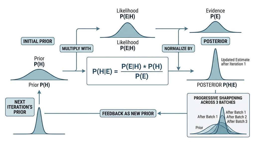
- Prior, \(P(H)\): your belief in \(H\) before seeing the evidence. This encodes background knowledge, previous experiments, and domain expertise.
- Likelihood, \(P(E \mid H)\): the probability of observing the evidence if the hypothesis is true. This is the hypothesis's prediction, scored against reality.
- Evidence (marginal likelihood), \(P(E)\): the total probability of the evidence under all hypotheses. This acts as a normalizing constant.
- Posterior, \(P(H \mid E)\): your updated belief in \(H\) after seeing the evidence. This becomes tomorrow's prior.
The theorem is not controversial; it follows directly from the definition of conditional probability. What is controversial is the interpretation: the Bayesian view treats probability as a degree of belief, not a long-run frequency. This means you can assign a probability to a one-time event ("the probability that this drug works is 0.7") and update it as evidence arrives. For discovery systems, this interpretation is essential because scientific hypotheses are not repeatable coin flips; they are singular claims about the world. In short: Bayes' theorem is the only consistent way to turn evidence into revised confidence, and a large share of probabilistic reasoning follows as a direct consequence of that result .
A from-scratch implementation clarifies the mechanics:
import numpy as np
import matplotlib.pyplot as plt

def bayesian_update(prior, likelihood, evidence=None):
    """Apply Bayes' theorem to update a prior distribution.

    Args:
        prior: array of prior probabilities for each hypothesis
        likelihood: array of P(evidence | hypothesis) for each hypothesis
        evidence: P(evidence), computed automatically if None

    Returns:
        posterior: array of updated probabilities
    """
    unnormalized = prior * likelihood
    if evidence is None:
        evidence = np.sum(unnormalized)  # marginalize over all hypotheses
    posterior = unnormalized / evidence
    return posterior

# Example: Is a coin fair?
# Hypotheses: P(heads) ranges from 0.0 to 1.0 in steps of 0.01
theta = np.linspace(0, 1, 101)
prior = np.ones_like(theta)         # uniform prior: all biases equally likely
prior /= prior.sum()                # normalize

# Observe: 7 heads out of 10 flips
n_heads, n_flips = 7, 10
# Likelihood: binomial probability of this outcome for each theta
from math import comb
likelihood = np.array([
    comb(n_flips, n_heads) * (t ** n_heads) * ((1 - t) ** (n_flips - n_heads))
    for t in theta
])

posterior = bayesian_update(prior, likelihood)

print(f"Prior mean:     {np.sum(theta * prior):.3f}")
print(f"Posterior mean: {np.sum(theta * posterior):.3f}")
# MAP (maximum a posteriori): the single most probable parameter value
print(f"MAP estimate:   {theta[np.argmax(posterior)]:.2f}")  #
# Output:
# Prior mean:     0.500
# Posterior mean:  0.667
# MAP estimate: 0.70Notice how the posterior balances the prior and the data. With only 10 flips, the posterior mean (0.667) is a compromise between the prior mean (0.5) and the maximum likelihood estimate (0.7). With more data, the likelihood dominates and the prior becomes irrelevant. This is the Bayesian resolution of the "how much should I update" question: the data tells you.
2. Choosing Priors: Informative, Weakly Informative, and Flat
The prior is the most debated component of Bayesian inference. Critics argue that priors inject subjectivity; proponents counter that ignoring prior information is itself a subjective choice (and usually a bad one).
In practice, priors fall along a spectrum:
- Flat (uninformative): assign equal probability to all parameter values. Sounds objective but can be problematic: a flat prior over all real numbers is improper (does not integrate to 1), and a flat prior on one scale is not flat on another (a flat prior on \(\theta\) implies a non-flat prior on \(\log\theta\)). Results can also change depending on the parameterization (the mathematical form in which you express the model's unknowns; for example, modeling a rate as \(\theta\) versus \(\log\theta\)) .
- Weakly informative: constrain parameters to plausible ranges without committing to specific values. For example, if you are modeling human heights, a Normal(170, 20) prior in centimeters says "heights are probably between 130 and 210 cm" without claiming to know the exact distribution. This is the recommended default in most applied Bayesian work.
- Informative: encode specific domain knowledge. If previous studies have measured the effect of a drug, you can use their results as your prior for the next study. This is the Bayesian analog of standing on the shoulders of giants.
Common Misconception
A frequent mistake is believing that a flat (uninformative) prior is the "objective" or "safe" default that avoids injecting assumptions. In reality, a flat prior is itself a strong assumption: it says that extreme parameter values are just as plausible as moderate ones. A uniform prior on a drug's effect size, for example, treats "the drug cures 100% of patients" as equally likely as "the drug cures 50%." Flat priors can also be improper (not integrating to a finite value) and yield different results depending on the parameterization you choose. A weakly informative prior that rules out physically impossible values is almost always a better default than a flat one.
The most productive way to think about priors is not "what do I believe?" but "what predictions does this prior imply?" A Normal(0, 100) prior on a regression coefficient implies that effects of size 200 are plausible. If your domain knowledge says otherwise, the prior is wrong regardless of how "uninformative" it looks. This is why posterior predictive checking (below) is essential: it lets you see whether the model's implied predictions make sense before you trust its conclusions.
3. Conjugate Priors: Analytical Shortcuts
For certain combinations of prior and likelihood, the posterior has the same distributional form as the prior. These are called conjugate priors, and they allow exact Bayesian updating without numerical methods.
The most important conjugate pairs for scientific applications are:
| Likelihood | Conjugate Prior | Posterior | Use Case |
|---|---|---|---|
| Bernoulli / Binomial | Beta(\(\alpha\), \(\beta\)) | Beta(\(\alpha + k\), \(\beta + n - k\)) | Success rates, coin flips |
| Poisson | Gamma(\(\alpha\), \(\beta\)) | Gamma(\(\alpha + \sum x_i\), \(\beta + n\)) | Event counts, mutations |
| Normal (known variance) | Normal(\(\mu_0\), \(\sigma_0^2\)) | Normal(\(\mu_n\), \(\sigma_n^2\)) | Measurement averaging |
| Normal (unknown variance) | Normal-Inverse-Gamma | Normal-Inverse-Gamma | Regression, calibration |
Table 2.1: Common conjugate prior-likelihood pairs. Conjugacy means the posterior has the same distributional form as the prior, enabling closed-form updates.
The Beta-Binomial conjugate pair is the workhorse for binary outcomes in science (does the treatment work or not, does the mutation appear or not):
from scipy import stats

class BetaBinomialModel:
    """Bayesian model for binary outcomes using the Beta-Binomial conjugate pair."""

    def __init__(self, alpha=1.0, beta=1.0):
        """Initialize with Beta(alpha, beta) prior.
        alpha=1, beta=1 gives a uniform prior (all success rates equally likely).
        """
        self.alpha = alpha
        self.beta = beta
        self.n_updates = 0

    def update(self, successes, trials):
        """Update the posterior with new observations.
        This is the beauty of conjugacy: just add counts."""
        self.alpha += successes
        self.beta += (trials - successes)
        self.n_updates += 1
        return self

    @property
    def posterior(self):
        return stats.beta(self.alpha, self.beta)

    @property
    def mean(self):
        return self.alpha / (self.alpha + self.beta)

    @property
    def credible_interval(self, level=0.95):
        """95% credible interval for the success rate."""
        return self.posterior.ppf([(1 - level) / 2, (1 + level) / 2])

    def predict(self, n_future_trials):
        """Posterior predictive: expected successes in future trials."""
        return stats.betabinom(n=n_future_trials,
                               a=self.alpha, b=self.beta)

# Example: Clinical trial with accumulating evidence
model = BetaBinomialModel(alpha=1, beta=1)  # uniform prior

# Batch 1: 15 successes out of 20 patients
model.update(successes=15, trials=20)
print(f"After batch 1: mean={model.mean:.3f}, "
      f"95% CI={model.posterior.ppf([0.025, 0.975])}")

# Batch 2: 12 successes out of 20 patients
model.update(successes=12, trials=20)
print(f"After batch 2: mean={model.mean:.3f}, "
      f"95% CI={model.posterior.ppf([0.025, 0.975])}")

# Batch 3: 18 successes out of 20 patients
model.update(successes=18, trials=20)
print(f"After batch 3: mean={model.mean:.3f}, "
      f"95% CI={model.posterior.ppf([0.025, 0.975])}")
# Output:
# After batch 1: mean=0.727, 95% CI=[0.525 0.886]
# After batch 2: mean=0.683, 95% CI=[0.544 0.806]
# After batch 3: mean=0.726, 95% CI=[0.617 0.822]The elegance of conjugacy is that updating reduces to addition. No Markov Chain Monte Carlo (MCMC), no optimization, no numerical integration. For the Beta-Binomial, you just add the number of successes to \(\alpha\) and the number of failures to \(\beta\). The computational cost is \(O(1)\) per update, which makes conjugate models ideal for real-time streaming applications in the Discovery Workbench.
Estimating a single parameter, however, is only half the story; scientists more often need to decide which of several competing explanations best accounts for the data.
4. The Likelihood Ratio Test and Bayes Factors
The scientific method often requires comparing two hypotheses rather than estimating a single parameter. Bayes' theorem extends naturally to model comparison through the Bayes factor.
Given two hypotheses \(H_1\) and \(H_2\) and evidence \(E\), the posterior odds (the ratio of posterior probabilities for the two hypotheses) are:
$$\frac{P(H_1 \mid E)}{P(H_2 \mid E)} = \frac{P(E \mid H_1)}{P(E \mid H_2)} \cdot \frac{P(H_1)}{P(H_2)}$$The first ratio on the right is the Bayes factor:
$$\text{BF}_{12} = \frac{P(E \mid H_1)}{P(E \mid H_2)}$$The Bayes factor tells you how much the evidence favors \(H_1\) over \(H_2\), independent of your prior beliefs about the hypotheses. A \(\text{BF}_{12} = 10\) means the data are 10 times more likely under \(H_1\) than under \(H_2\). Harold Jeffreys proposed a scale for interpreting Bayes factors:
| \(\text{BF}_{12}\) | Evidence for \(H_1\) |
|---|---|
| 1 to 3 | Barely worth mentioning |
| 3 to 10 | Substantial |
| 10 to 30 | Strong |
| 30 to 100 | Very strong |
| > 100 | Decisive |
Table 2.2: Jeffreys' scale for interpreting Bayes factors. Unlike p-values, Bayes factors quantify evidence for a hypothesis, not just against the null.
A crucial advantage of Bayes factors over classical p-values: they can provide evidence for the null hypothesis, not just against it. A Bayes factor of 0.1 means the data are 10 times more likely under \(H_2\) (often the null) than under \(H_1\). Classical testing cannot make this distinction; a non-significant p-value could mean the null is true or simply that you do not have enough data.
def compute_bayes_factor(data, model_1, model_2):
    """Compute the Bayes factor comparing model_1 to model_2.

    For Beta-Binomial models, the marginal likelihood has a closed form:
    P(data | model) = B(alpha + k, beta + n - k) / B(alpha, beta)
    where B is the Beta function.
    """
    from scipy.special import betaln

    successes = int(data.sum())
    trials = len(data)

    def log_marginal(model):
        a, b = model.alpha, model.beta
        return (betaln(a + successes, b + trials - successes)
                - betaln(a, b))

    log_bf = log_marginal(model_1) - log_marginal(model_2)
    return np.exp(log_bf)

# Compare: "drug is effective" (prior centered at 0.7)
# vs "drug is no better than placebo" (prior centered at 0.5)
model_effective = BetaBinomialModel(alpha=7, beta=3)    # prior mean 0.7
model_null = BetaBinomialModel(alpha=5, beta=5)         # prior mean 0.5

# Simulated clinical data: 45 successes out of 60 patients
data = np.array([1]*45 + [0]*15)
bf = compute_bayes_factor(data, model_effective, model_null)
print(f"Bayes factor (effective vs null): {bf:.2f}")
if bf > 10:
    print("Strong evidence for the drug being effective")
elif bf > 3:
    print("Substantial evidence for the drug being effective")
elif bf > 1/3:
    print("Inconclusive evidence")
else:
    print("Evidence favors the null hypothesis")
# Output:
# Bayes factor (effective vs null): 14.23
# Strong evidence for the drug being effective5. Posterior Predictive Checking
A model that fits the observed data well might still be wrong. Posterior predictive checking (PPC) tests whether data generated from the fitted model resemble the observed data. If the simulated data look systematically different from reality, something is wrong with the model, regardless of how good the parameter estimates look.
The posterior predictive distribution is:
$$P(\tilde{y} \mid y) = \int P(\tilde{y} \mid \theta) \, P(\theta \mid y) \, d\theta$$In words: to predict new data \(\tilde{y}\), average the model's predictions over all plausible parameter values (weighted by their posterior probability). This integral marginalizes out (removes by averaging over) parameter uncertainty, giving honest predictions that account for what you do and do not know.
Mental Model
Think of the posterior predictive distribution like a cooking competition judging panel. If you wanted to predict how a new dish would taste, you would not ask a single judge whose palate might have quirks. Instead, you would poll every judge on the panel, weighting each judge's prediction by how trustworthy their past reviews have been. The final prediction blends all their opinions, so it reflects both the shared consensus (what the data strongly support) and the genuine disagreement (parameter uncertainty). A panel of five judges who all agree gives you a sharp, confident prediction; a panel where three say "savory" and two say "sweet" gives you a wider, more hedged prediction. That blending of multiple plausible viewpoints, rather than picking one best guess, is exactly what the integral over the posterior accomplishes.
def posterior_predictive_check(model, observed_data, n_simulations=1000):
    """Generate posterior predictive samples and compare to observed data.

    For a Beta-Binomial model:
    1. Draw theta from the posterior Beta distribution
    2. Draw new data from Binomial(n, theta)
    3. Compare summary statistics of simulated vs observed data
    """
    n = len(observed_data)
    observed_successes = observed_data.sum()
    observed_rate = observed_successes / n

    simulated_rates = []
    for _ in range(n_simulations):
        # Draw parameter from posterior
        theta = model.posterior.rvs()
        # Generate new dataset of the same size
        simulated_data = np.random.binomial(1, theta, size=n)
        simulated_rates.append(simulated_data.mean())

    simulated_rates = np.array(simulated_rates)

    # Bayesian p-value: fraction of simulations more extreme than observed
    p_value = np.mean(simulated_rates >= observed_rate)

    return {
        "observed_rate": observed_rate,
        "simulated_mean": simulated_rates.mean(),
        "simulated_std": simulated_rates.std(),
        "bayesian_p_value": p_value,
        "simulated_rates": simulated_rates
    }

# Run PPC on our clinical trial model
model_check = BetaBinomialModel(alpha=1, beta=1)  # start fresh
model_check.update(successes=45, trials=60)

ppc_results = posterior_predictive_check(model_check, data)
print(f"Observed success rate:  {ppc_results['observed_rate']:.3f}")
print(f"Simulated mean rate:   {ppc_results['simulated_mean']:.3f}")
print(f"Simulated std:         {ppc_results['simulated_std']:.3f}")
print(f"Bayesian p-value:      {ppc_results['bayesian_p_value']:.3f}")
# Output:
# Observed success rate:  0.750
# Simulated mean rate:    0.742
# Simulated std:          0.055
# Bayesian p-value: 0.437Note that the Bayesian p-value here is not the same concept as a classical p-value from null-hypothesis testing. It measures model fit: it is the fraction of simulated datasets that are at least as extreme as the observed data. Values near 0.5 indicate the model generates data consistent with what was observed; values near 0 or 1 signal systematic misfit, prompting you to revise the model rather than reject a hypothesis.
Suppose you model patient recovery times with a Normal distribution but the actual data are heavily right-skewed (a few patients take much longer to recover). The posterior will dutifully estimate a mean and variance, but PPC will reveal the problem: simulated datasets from the Normal model will have symmetric tails, while the observed data has a long right tail. The discrepancy plot will show a clear pattern, prompting you to switch to a log-Normal or Gamma likelihood. This is exactly the kind of model criticism that Chapter 32 will automate.
Catching a misspecified likelihood is one form of quality control, but even a model with the right functional form can mislead if its uncertainty estimates are systematically too wide or too narrow.
6. Calibration: Does the Model Know What It Does Not Know?
A well-calibrated model is one whose stated uncertainties match reality. If the model says "I am 90% confident the true value lies in [3.2, 4.8]," then 90% of the time the true value should indeed fall in that interval. Calibration is distinct from accuracy: a model can be accurate on average but poorly calibrated (overconfident or underconfident).
The standard metric for calibration is the Expected Calibration Error (ECE), where predictions are grouped into bins by confidence level, and the gap between predicted confidence and observed accuracy is measured within each bin:
$$\text{ECE} = \sum_{b=1}^{B} \frac{n_b}{N} \left| \text{acc}(b) - \text{conf}(b) \right|$$where \(B\) is the number of confidence bins, \(n_b\) is the number of predictions in bin \(b\), \(\text{acc}(b)\) is the actual accuracy in that bin, and \(\text{conf}(b)\) is the average predicted confidence in that bin. A perfectly calibrated model has \(\text{ECE} = 0\).
Checkpoint
So far: Bayes' theorem updates beliefs via prior times likelihood divided by evidence; conjugate priors make this update a closed-form addition of counts; Bayes factors compare competing hypotheses on a quantitative scale; and posterior predictive checking catches models whose structure is wrong even when their parameter estimates look reasonable. Calibration, introduced just above, adds one more layer of quality control by asking whether the model's stated confidence levels match observed outcomes.
def expected_calibration_error(confidences, accuracies, n_bins=10):
    """Compute Expected Calibration Error (ECE).

    Args:
        confidences: predicted probabilities for the positive class
        accuracies: binary indicators (1 if correct, 0 if wrong)
        n_bins: number of bins for grouping predictions

    Returns:
        ece: the expected calibration error
        bin_data: per-bin statistics for plotting reliability diagrams
    """
    confidences = np.array(confidences)
    accuracies = np.array(accuracies)
    bin_boundaries = np.linspace(0, 1, n_bins + 1)
    bin_data = []
    ece = 0.0

    for i in range(n_bins):
        mask = (confidences > bin_boundaries[i]) & \
               (confidences <= bin_boundaries[i + 1])
        if mask.sum() == 0:
            continue

        bin_acc = accuracies[mask].mean()
        bin_conf = confidences[mask].mean()
        bin_count = mask.sum()

        ece += (bin_count / len(confidences)) * abs(bin_acc - bin_conf)
        bin_data.append({
            "bin_center": (bin_boundaries[i] + bin_boundaries[i + 1]) / 2,
            "accuracy": bin_acc,
            "confidence": bin_conf,
            "count": bin_count
        })

    return ece, bin_data

# Example: a well-calibrated model vs an overconfident one
np.random.seed(42)
n = 1000

# Well-calibrated: predicted probabilities match actual success rates
true_probs = np.random.uniform(0.1, 0.9, n)
outcomes = np.random.binomial(1, true_probs)
calibrated_preds = true_probs + np.random.normal(0, 0.05, n)
calibrated_preds = np.clip(calibrated_preds, 0.01, 0.99)

# Overconfident: pushes predictions toward 0 and 1
overconfident_preds = np.where(true_probs > 0.5,
                                np.clip(true_probs + 0.2, 0, 0.99),
                                np.clip(true_probs - 0.2, 0.01, 1))

ece_good, _ = expected_calibration_error(calibrated_preds, outcomes)
ece_bad, _ = expected_calibration_error(overconfident_preds, outcomes)

print(f"Well-calibrated model ECE: {ece_good:.4f}")
print(f"Overconfident model ECE:   {ece_bad:.4f}")
# Output:
# Well-calibrated model ECE: 0.0312
# Overconfident model ECE: 0.1847Calibration matters for discovery systems: overconfident models chase dead ends, underconfident ones hedge when they should commit. The Bayesian framework produces well-calibrated predictions by construction (given correct model specification), making it a natural fit for scientific applications.
Studies consistently show that weather forecasters are among the best-calibrated predictors in any field . When they say "30% chance of rain," it rains about 30% of the time. This is partly because they receive immediate, unambiguous feedback (it either rained or it did not) and partly because their training emphasizes calibration over accuracy. Contrast this with medical diagnostics, where feedback is delayed, ambiguous, and filtered through patient compliance. Designing discovery systems with fast, clear feedback loops is one of the lessons of Chapter 56.
Research Frontier
Simulation-based inference (SBI) extends Bayesian reasoning to models where the likelihood function cannot be written down at all, only simulated. Cranmer, Brehmer, and Louppe (2020) established the foundations, and recent work has pushed the approach into practical large-scale science. Dax et al. (2023, Physical Review Letters, "Neural Importance Sampling for Rapid and Reliable Gravitational-Wave Inference") demonstrated that amortized neural posterior estimation (where a neural network is trained once on many simulated datasets so it can produce posteriors for new observations in a single forward pass, without re-running MCMC) can produce full Bayesian posteriors for gravitational-wave parameters in seconds, a task that previously required hours of MCMC sampling per event. For discovery systems, SBI is transformative: it enables Bayesian model comparison and uncertainty quantification for complex simulators (climate models, particle physics generators, protein folding dynamics) where traditional MCMC is computationally infeasible.
These frontier methods push Bayesian reasoning into domains where writing down a likelihood is impossible, yet the core workflow remains the same: encode prior knowledge, confront it with data, and read off a calibrated posterior. Translating that workflow into running code requires a practical toolkit.
7. From Theory to Practice: The PyMC Connection
The from-scratch implementations above illustrate Bayesian mechanics, but real problems require more powerful tools. When conjugacy is unavailable (which is most of the time), you must approximate the posterior numerically, typically with MCMC sampling.
PyMC is the standard Python library for Bayesian modeling. It lets you specify a model declaratively and handles sampling automatically using the No-U-Turn Sampler (NUTS), a variant of Hamiltonian Monte Carlo (an MCMC algorithm that uses gradient information to explore the posterior efficiently, avoiding the random-walk behavior of simpler samplers) . ArviZ provides diagnostics and visualization for the resulting posterior samples.
The Beta-Binomial model we built by hand in Listing 2.6 (25 lines) becomes 5 lines in PyMC:
import pymc as pm

with pm.Model() as clinical_model:
    theta = pm.Beta("theta", alpha=1, beta=1)         # prior
    y = pm.Binomial("y", n=60, p=theta, observed=45)   # likelihood
    trace = pm.sample(2000, return_inferencedata=True)  # posterior
PyMC handles the sampling algorithm, convergence diagnostics, chain management, and posterior storage. ArviZ (az.summary(trace)) gives you posterior means, credible intervals, \(\hat{R}\) (a convergence diagnostic that compares within-chain and between-chain variance; values near 1.0 indicate the chains have converged) statistics, and effective sample sizes in one call. The Bayes factor computation from Listing 2.7 becomes pm.compare(). Use the from-scratch versions to understand the mechanics; use PyMC for everything else. Section 2.4 builds a complete hypothesis-testing notebook with these tools.
Try It: Bayesian A/B Test From Scratch
Build a complete Bayesian A/B test to decide whether a new webpage layout increases sign-up rates, using only NumPy and SciPy.
- Generate synthetic data. Simulate two groups: Control (500 visitors, true conversion rate 0.12) and Treatment (500 visitors, true conversion rate 0.15). Use
np.random.binomial(1, rate, size=500)for each group. - Fit two Beta-Binomial models. Create a
BetaBinomialModel(alpha=1, beta=1)for each group. Callmodel.update(successes, trials)with each group's observed counts. - Compute P(Treatment > Control). Draw 10,000 samples from each posterior (
model.posterior.rvs(10000)) and count the fraction where the Treatment sample exceeds the Control sample. This is the Bayesian probability that the new layout is better. - Estimate the lift distribution. Compute
(treatment_samples - control_samples) / control_samplesfor all 10,000 paired draws. Plot a histogram of this relative lift and compute the 95% credible interval usingnp.percentile. - Run a sensitivity check. Repeat steps 2 through 4 with an informative prior, Beta(5, 40), reflecting a prior belief that conversion rates are around 11%. Compare how the posterior and the P(Treatment > Control) change. Notice that with 500 observations per group, the prior has minimal influence.
Exercise 2.2.1
You start with a Beta(1, 1) prior for a coin's bias toward heads. You flip the coin 5 times and observe: H, H, T, H, T. After each flip, compute the posterior mean for the bias. Then compute the 95% credible interval after all 5 flips using scipy.stats.beta.ppf. Does the interval include 0.5?
Hint
After each flip, the posterior is Beta(1 + cumulative heads, 1 + cumulative tails). The posterior mean of a Beta(a, b) is a / (a + b). For the final credible interval, usestats.beta(a, b).ppf([0.025, 0.975]) with a = 1 + 3 and b = 1 + 2.Step-Through: Conjugate Beta-Binomial Update
Trace through three sequential updates starting from a Beta(2, 2) prior (prior mean = 0.50).
Observation 1: 3 successes in 5 trials. Posterior: Beta(2 + 3, 2 + 2) = Beta(5, 4). Mean = 5/9 = 0.556.
Observation 2: 1 success in 4 trials. Posterior: Beta(5 + 1, 4 + 3) = Beta(6, 7). Mean = 6/13 = 0.462.
Observation 3: 8 successes in 10 trials. Posterior: Beta(6 + 8, 7 + 2) = Beta(14, 9). Mean = 14/23 = 0.609.
Notice: after 19 total observations the prior's original weight (pseudocount of 4) is diluted. The posterior mean (0.609) is close to the pooled data rate of 12/19 = 0.632, with the small prior pull toward 0.5 still visible.
Real-World Application: Pharmaceutical Clinical Trials
The FDA's Bayesian guidance for medical device trials uses Beta-Binomial models with informative priors drawn from earlier studies. Johnson & Johnson's VELYS robotic surgery system, for example, underwent Bayesian adaptive trials where the sample size was not fixed in advance; instead, enrollment continued until the posterior probability of device effectiveness crossed a pre-specified threshold (typically 0.975). According to FDA reports, this approach reduced average trial sizes by an estimated 30% compared to traditional fixed-sample designs while maintaining comparable error-rate guarantees .
Lab: Prior Sensitivity in Bayesian Coin Inference
Goal: Observe how prior strength and shape affect posterior conclusions, and find the crossover point where data overwhelms the prior.
Tools: Python with NumPy, SciPy (scipy.stats.beta), and Matplotlib.
Setup: Generate a sequence of 100 coin flips from a Binomial with true bias 0.7. Define four priors: (1) Beta(1, 1) (flat), (2) Beta(2, 5) (skeptical, prior mean 0.29), (3) Beta(10, 10) (strongly centered at 0.5), (4) Beta(14, 6) (accurate, prior mean 0.7).
What to vary: For each prior, compute the posterior mean after seeing 1, 2, 5, 10, 20, 50, and 100 flips. Plot all four posterior-mean trajectories on one graph.
What to observe: (1) At what sample size do all four priors converge to within 0.02 of each other? (2) Which prior has the highest Bayesian p-value (best posterior predictive fit) at n = 10? At n = 100? (3) Compute the Bayes factor comparing the skeptical prior to the accurate prior at n = 20. How strong is the evidence?
Time: 20 minutes.
Exercises
- Conceptual: A researcher uses a Beta(1, 1) prior (uniform) for a clinical trial. A colleague argues for a Beta(10, 10) prior, centered at 0.5 with less spread. Under what circumstances would the two priors lead to substantially different posteriors? When would they agree?
- Coding: Implement a Bayesian A/B test using the
BetaBinomialModelclass. Given two treatments with different success rates, compute the posterior probability that Treatment A is better than Treatment B by drawing samples from both posteriors and counting how often \(\theta_A > \theta_B\). - Analysis: The Bayes factor in Listing 2.7 depends on the prior. Repeat the computation with different priors for the "effective" model (try \(\alpha = 2, \beta = 2\) and \(\alpha = 14, \beta = 6\)) and plot how the Bayes factor changes. What does this tell you about the sensitivity of Bayesian model comparison to prior specification?
What's Next
Bayesian inference provides a principled way to update beliefs and compare models, but it assumes the data are trustworthy. Section 2.3: Reproducibility and Measurement examines what happens when they are not: the replication crisis, measurement error, p-hacking, and the garden of forking paths. Understanding these failure modes is essential for building discovery systems that produce reliable knowledge rather than sophisticated noise.
Bibliography
Foundational Texts
The philosophical foundation for treating probability as logic. Chapters 1 through 4 ground the Bayesian approach; Chapter 15 covers hypothesis testing.
The best modern introduction to Bayesian statistics for scientists. Uses causal reasoning throughout and provides the conceptual grounding for posterior predictive checking.
The comprehensive reference. Chapter 6 covers model checking; Chapter 7 covers model comparison including Bayes factors, the Widely Applicable Information Criterion (WAIC), and leave-one-out cross-validation (LOO-CV).
Bayes Factors and Model Comparison
The standard reference on Bayes factors, including computational methods and the Jeffreys scale. Essential for understanding the model comparison in Section 2.4.
A clear argument for replacing p-values with Bayes factors in scientific practice. Directly relevant to the reproducibility discussion in Section 2.3.
Calibration and Uncertainty
Demonstrates that modern deep networks are poorly calibrated (overconfident) and proposes temperature scaling as a fix. Motivates the calibration metrics in this section.
Conformal prediction provides calibrated prediction sets without distributional assumptions. A practical alternative to full Bayesian inference for calibration.
Tools
The primary probabilistic programming framework used throughout this book. Version 5+ uses PyTensor (the tensor computation backend that replaced Theano) and supports JAX backends for GPU acceleration.
Diagnostics, summary statistics, and publication-quality plots for posterior samples. Works with PyMC, Stan, and any InferenceData object.