5.2 Simulation and Surrogate Models

"I can simulate the entire universe. It just takes slightly longer than the universe itself. Hence the surrogate."

A Finite Element Mesh Contemplating Its Budget

1. Simulation as the Third Pillar of Science

What would it take to test ten thousand wing designs, screen a million drug candidates, or forecast a century of climate change before committing to a single physical prototype? Simulation stands apart from the other modes of discovery introduced in Section 5.1. It originates from theory (you implement the equations) but generates synthetic data as output. A simulation is a computational experiment, a controlled investigation where you vary inputs and observe outputs without touching the physical world.

What. A simulator is a deterministic or stochastic function \(f: \mathcal{X} \to \mathcal{Y}\) that maps input parameters (design variables, initial conditions, physical constants) to output quantities of interest (stress, yield, binding energy, climate trajectory). The function \(f\) encodes a theory, but evaluating it requires computation rather than algebra.

Why. Simulations enable discovery in domains where experiments are impractical. You cannot crash ten thousand cars to optimize a bumper design. You cannot wait centuries to test climate policy. You cannot synthesize every conceivable molecule to find a drug. Simulation lets you explore these spaces computationally.

How. Discretize the governing equations (finite elements, finite differences, molecular dynamics), set up boundary and initial conditions, run the solver, post-process the results. Each run produces one data point in the space of possible experiments.

When. Use simulation when the governing equations are known but analytically intractable, when real experiments are too costly or dangerous, or when you need to explore a vast parameter space before committing to physical prototypes.

The concept of a digital twin, a continuously updated simulation model of a specific physical system, extends the simulation paradigm from exploration to monitoring. A digital twin of a jet engine ingests sensor data in real time, updates its parameters, and predicts remaining useful life. We revisit digital twins in Chapter 43: Scientific Simulation.

2. The Cost Problem and the Surrogate Solution

The fundamental bottleneck is cost. A high-fidelity CFD simulation of airflow around an aircraft wing might take 48 hours on 1,000 cores. If your design space has 20 parameters and you want to map the response surface, even a sparse Latin hypercube design requires 200 points. At 48 hours per simulation, that totals over a year of wall-clock time on a major cluster.

Without a faster alternative, engineers face an impossible choice: either explore the design space so sparsely that they miss the best solutions, or blow through months of compute budget on a single optimization campaign. In one widely cited case, a Formula 1 aerodynamics team reportedly abandoned a promising front-wing concept because the CFD queue could not turn results around before the regulatory deadline.

A surrogate model (also called a metamodel, response surface, or emulator) is a cheap approximation \(\hat{f}\) trained on a small set of simulation evaluations \(\mathcal{D} = \{(\mathbf{x}_i, f(\mathbf{x}_i))\}_{i=1}^{N}\). Once trained, the surrogate can be evaluated in milliseconds, enabling tasks that require thousands or millions of evaluations: optimization, sensitivity analysis, uncertainty propagation, and active learning. That gap, from 48 hours per simulation to a few milliseconds per surrogate query, represents a speedup of roughly six orders of magnitude, enough to turn a year-long parameter sweep into an afternoon's computation.

A surrogate model approximates the input-output mapping of an expensive simulator by interpolating a small training set of exact evaluations. Instead of running the simulator millions of times, you run it tens or hundreds of times, fit a surrogate, and query it at negligible cost. The surrogate exploits patterns in the training data (smoothness, periodicity, monotonicity) to predict outputs at untested inputs. Use a surrogate when each evaluation costs minutes to days and downstream tasks require many evaluations; use the full simulator when evaluations are cheap or guaranteed fidelity is essential.

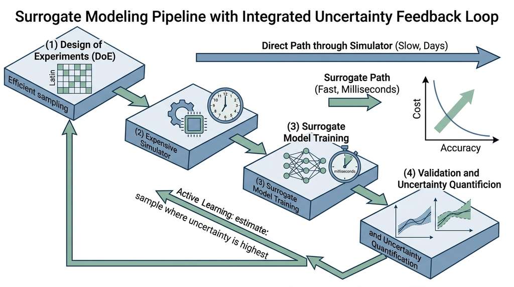
The surrogate modeling pipeline has four stages, illustrated in Figure 5.2:

1. Design of experiments (DoE): Choose an initial set of input points \(\{\mathbf{x}_i\}\) that covers the parameter space efficiently. Common strategies include Latin hypercube sampling (where each parameter's range is divided into equal intervals and exactly one sample is placed in each interval per dimension), Sobol sequences (low-discrepancy quasi-random sequences that fill the space more uniformly than pseudorandom samples), and space-filling designs.
2. Simulation: Run the expensive simulator at each design point to obtain \(\{f(\mathbf{x}_i)\}\).
3. Fitting: Train the surrogate \(\hat{f}\) on the (input, output) pairs.
4. Validation: Assess surrogate accuracy on held-out simulation runs and quantify prediction uncertainty. Figure 5.2.1 illustrates surrogate modeling pipeline with uncertainty feedback loop.

Let us build a surrogate for a simple but instructive test function: the Branin function, a standard benchmark in surrogate modeling and Bayesian optimization. In short: a surrogate trades a small, upfront investment in simulation runs for the ability to explore millions of designs at near-zero marginal cost, but only if you can quantify where its predictions go wrong.

import numpy as np
from scipy.stats import qmc

def branin(x1, x2):
    """Branin test function (3 global minima)."""
    a, b, c = 1.0, 5.1 / (4 * np.pi**2), 5.0 / np.pi
    r, s, t = 6.0, 10.0, 1.0 / (8 * np.pi)
    return a * (x2 - b*x1**2 + c*x1 - r)**2 + s*(1 - t)*np.cos(x1) + s

# Stage 1: Latin Hypercube design (20 points in 2D)
sampler = qmc.LatinHypercube(d=2, seed=42)
sample = sampler.random(n=20)
# Scale to Branin domain: x1 in [-5, 10], x2 in [0, 15]
l_bounds = np.array([-5, 0])
u_bounds = np.array([10, 15])
X_train = qmc.scale(sample, l_bounds, u_bounds)

# Stage 2: Evaluate the "expensive" simulator
y_train = np.array([branin(x[0], x[1]) for x in X_train])

print(f"Training set: {len(X_train)} points")
print(f"Output range: [{y_train.min():.2f}, {y_train.max():.2f}]")
print(f"Known global minimum: ~0.398 at three locations")

Training set: 20 points
Output range: [1.01, 236.73]
Known global minimum: ~0.398 at three locations

3. Types of Surrogate Models

Several model families serve as surrogates, each with distinct trade-offs in flexibility, data efficiency, and uncertainty quantification:

Polynomial response surfaces. The oldest approach: fit a low-degree polynomial (typically quadratic) to the simulation data. Fast to train, easy to interpret, but they cannot capture complex, multimodal response landscapes. The quadratic model for \(d\) inputs has \(\binom{d+2}{2}\) parameters, so even in moderate dimensions the number of required simulations grows quickly.

Radial basis functions (RBFs). Interpolate the data exactly using a sum of radially symmetric basis functions centered at the training points: \(\hat{f}(\mathbf{x}) = \sum_{i=1}^{N} w_i \phi(\|\mathbf{x} - \mathbf{x}_i\|)\). Common choices for \(\phi\) include Gaussian, multiquadric, and thin-plate spline kernels. RBFs scale well to moderate dimensions and handle irregular data layouts.

Probabilistic and learned surrogates

Gaussian processes (GPs). The workhorse of modern surrogate modeling. A GP places a distribution over functions, providing not just a prediction \(\mu(\mathbf{x})\) but also a predictive variance \(\sigma^2(\mathbf{x})\) that quantifies uncertainty. We develop GPs in detail in Section 5.3.

Neural network surrogates. Deep neural networks can approximate arbitrarily complex functions and scale to high-dimensional inputs. Their weakness for surrogate modeling is that standard neural networks do not provide calibrated uncertainty estimates. Ensembles and Bayesian neural networks (discussed below) address this gap.

Let us fit both a polynomial and an RBF surrogate to our Branin data, then compare their predictions.

import numpy as np
from sklearn.preprocessing import PolynomialFeatures
from sklearn.linear_model import LinearRegression
from sklearn.pipeline import make_pipeline
from scipy.interpolate import RBFInterpolator

# Polynomial surrogate (degree 2)
poly_model = make_pipeline(
    PolynomialFeatures(degree=2, include_bias=True),
    LinearRegression()
)
poly_model.fit(X_train, y_train)

# RBF surrogate (thin-plate spline)
rbf_model = RBFInterpolator(X_train, y_train, kernel='thin_plate_spline')

# Evaluate on a dense test grid
n_grid = 50
x1_grid = np.linspace(-5, 10, n_grid)
x2_grid = np.linspace(0, 15, n_grid)
X1, X2 = np.meshgrid(x1_grid, x2_grid)
X_test = np.column_stack([X1.ravel(), X2.ravel()])

y_true = np.array([branin(x[0], x[1]) for x in X_test])
y_poly = poly_model.predict(X_test)
y_rbf = rbf_model(X_test)

# Compute errors
rmse_poly = np.sqrt(np.mean((y_poly - y_true)**2))
rmse_rbf = np.sqrt(np.mean((y_rbf - y_true)**2))

print(f"Polynomial (deg 2) RMSE: {rmse_poly:.2f}")
print(f"RBF (thin plate)   RMSE: {rmse_rbf:.2f}")
print(f"RBF is {rmse_poly/rmse_rbf:.1f}x more accurate than polynomial")

Polynomial (deg 2) RMSE: 29.14
RBF (thin plate)   RMSE: 5.83
RBF is 5.0x more accurate than polynomial

4. Epistemic Uncertainty: Knowing What You Don't Know

Prediction uncertainty comes in two flavors, a distinction with roots in decision theory and structural engineering, examined rigorously by Der Kiureghian and Ditlevsen (2009) and popularized for deep learning by Kendall and Gal (2017):

Aleatoric uncertainty (from Latin alea, "dice") captures irreducible randomness in the data. If you measure a patient's blood pressure ten times, the readings will vary due to biological fluctuations, sensor noise, and other sources beyond your control. No amount of additional data eliminates aleatoric uncertainty; it is a property of the phenomenon itself.

Epistemic uncertainty (from Greek episteme, "knowledge") captures reducible ignorance about the model. If you have observed a function at five points and want to predict at a sixth, your uncertainty is high because you lack information, not because the function is random. Collecting one more data point at the right location can dramatically reduce epistemic uncertainty.

The total predictive variance decomposes as:

For surrogate models of deterministic simulators, aleatoric uncertainty is zero (the simulator produces the same output every time for the same input). All uncertainty is epistemic: it reflects the surrogate's ignorance about the true function in regions far from training data. This makes epistemic uncertainty the ideal guide for deciding where to sample next, the core idea behind active learning (Section 5.3).

5. Quantifying Uncertainty: Ensembles

The simplest approach to epistemic uncertainty: train multiple models on the same data (with different random seeds, architectures, or data subsets) and measure their disagreement. Where the models agree, you can be confident. Where they disagree, you know the prediction is uncertain.

For an ensemble of \(M\) models \(\{\hat{f}_1, \ldots, \hat{f}_M\}\), the ensemble mean and variance at a point \(\mathbf{x}\) are:

This ensemble variance is a practical estimate of epistemic uncertainty. Lakshminarayanan et al. (2017) showed that deep ensembles provide well-calibrated uncertainty estimates with minimal implementation overhead.

import numpy as np
from sklearn.neural_network import MLPRegressor

# Train an ensemble of 10 neural network surrogates
M = 10
ensemble = []
for m in range(M):
    nn = MLPRegressor(
        hidden_layer_sizes=(64, 32),
        max_iter=2000,
        random_state=m,        # different initialization
        learning_rate_init=0.01,
        early_stopping=True,
        validation_fraction=0.2
    )
    nn.fit(X_train, y_train)
    ensemble.append(nn)

# Predict on test grid
predictions = np.array([nn.predict(X_test) for nn in ensemble])
mu_ens = predictions.mean(axis=0)
sigma_ens = predictions.std(axis=0)

# RMSE of ensemble mean
rmse_ens = np.sqrt(np.mean((mu_ens - y_true)**2))
print(f"Ensemble mean RMSE: {rmse_ens:.2f}")

# Where is uncertainty highest?
top5_idx = np.argsort(sigma_ens)[-5:]
print("\nHighest uncertainty locations:")
for idx in top5_idx:
    print(f"  x=({X_test[idx,0]:.1f}, {X_test[idx,1]:.1f}), "
          f"std={sigma_ens[idx]:.1f}, "
          f"true={y_true[idx]:.1f}, pred={mu_ens[idx]:.1f}")

Ensemble mean RMSE: 8.47

Highest uncertainty locations:
  x=(10.0, 0.0), std=42.3, true=236.7, pred=194.1
  x=(10.0, 0.6), std=38.7, true=204.5, pred=167.2
  x=(-5.0, 0.0), std=35.1, true=108.2, pred=72.8
  x=(9.7, 0.0), std=33.9, true=223.4, pred=190.6
  x=(-5.0, 0.6), std=31.4, true=83.4, pred=53.1

Practical Example: Ensemble Surrogates in Drug Discovery

At AstraZeneca and other pharmaceutical companies, ensemble neural networks serve as surrogates for molecular dynamics simulations of protein-ligand binding. Each binding free energy calculation takes hours on a GPU cluster; the ensemble surrogate predicts binding affinity in milliseconds and flags uncertain predictions for full simulation. Molecules where the ensemble disagrees are prioritized for expensive calculations, a form of active learning that can reduce the simulation budget by an estimated 5 to 10 times compared to uniform sampling. Variants of this approach were evaluated in the 2023 CACHE challenge for computer-aided drug design.

6. Quantifying Uncertainty: Bayesian Neural Networks

Ensembles approximate epistemic uncertainty by training multiple models. Bayesian neural networks (BNNs), where the network's weights are treated as random variables with a learned posterior distribution rather than fixed point estimates, take a more principled approach: instead of learning point estimates for the weights \(\mathbf{w}\), they learn a posterior distribution \(p(\mathbf{w} \mid \mathcal{D})\). The predictive distribution at a new point \(\mathbf{x}^*\) integrates over all plausible weight settings:

This integral is intractable for all but trivial networks, so practitioners use approximations. The two most popular are:

Monte Carlo Dropout (Gal and Ghahramani, 2016). Keep dropout active at test time and run the network \(T\) times. The resulting predictions approximate samples from the posterior predictive distribution (the distribution of outputs after integrating over model uncertainty, as opposed to a single best-guess prediction). This requires zero architectural changes to a standard dropout network.

Variational inference (an optimization-based approximation technique that replaces an intractable integral with a simpler, tunable distribution fitted to mimic the true posterior). Approximate \(p(\mathbf{w} \mid \mathcal{D})\) with a tractable distribution \(q_\phi(\mathbf{w})\) (typically a diagonal Gaussian) by minimizing the Kullback-Leibler (KL) divergence. The Bayes by Backprop algorithm (Blundell et al., 2015) does this with standard gradient descent.

import torch
import torch.nn as nn

class MCDropoutSurrogate(nn.Module):
    """Neural network surrogate with MC Dropout for uncertainty."""
    def __init__(self, input_dim=2, hidden=64, dropout_rate=0.1):
        super().__init__()
        self.net = nn.Sequential(
            nn.Linear(input_dim, hidden),
            nn.ReLU(),
            nn.Dropout(dropout_rate),
            nn.Linear(hidden, hidden),
            nn.ReLU(),
            nn.Dropout(dropout_rate),
            nn.Linear(hidden, 1)
        )

    def forward(self, x):
        return self.net(x).squeeze(-1)

    def predict_with_uncertainty(self, x, n_samples=100):
        """Run n_samples forward passes with dropout active."""
        self.train()  # keep dropout ON
        with torch.no_grad():
            preds = torch.stack([self(x) for _ in range(n_samples)])
        mean = preds.mean(dim=0)
        std = preds.std(dim=0)
        return mean, std

# Train the MC Dropout model
torch.manual_seed(42)
X_t = torch.tensor(X_train, dtype=torch.float32)
y_t = torch.tensor(y_train, dtype=torch.float32)

model = MCDropoutSurrogate(dropout_rate=0.1)
optimizer = torch.optim.Adam(model.parameters(), lr=0.01)
loss_fn = nn.MSELoss()

for epoch in range(1000):
    model.train()
    pred = model(X_t)
    loss = loss_fn(pred, y_t)
    optimizer.zero_grad()
    loss.backward()
    optimizer.step()

# Predict with uncertainty
X_test_t = torch.tensor(X_test, dtype=torch.float32)
mu_mc, sigma_mc = model.predict_with_uncertainty(X_test_t, n_samples=200)

print(f"MC Dropout RMSE: "
      f"{torch.sqrt(torch.mean((mu_mc - torch.tensor(y_true, dtype=torch.float32))**2)):.2f}")
print(f"Mean uncertainty: {sigma_mc.mean():.2f}")
print(f"Max uncertainty:  {sigma_mc.max():.2f}")

MC Dropout RMSE: 12.34
Mean uncertainty: 8.71
Max uncertainty:  45.62

7. Surrogate Accuracy and the Exploration-Exploitation Trade-off

Epistemic uncertainty estimates become actionable when they guide where to allocate a limited simulation budget. A surrogate is only useful if you know where to trust it. The relationship between surrogate accuracy and the number of training simulations follows a characteristic curve: rapid improvement with the first few points, then diminishing returns. The key question for discovery is not "how accurate is the surrogate on average?" but "where is the surrogate most wrong, and should we sample there next?"

This question connects directly to the exploration-exploitation trade-off that we first encountered in Chapter 1:

• Exploitation: sample where the surrogate predicts the best outcome (lowest cost, highest yield, strongest binding).
• Exploration: sample where the surrogate is most uncertain, to improve the model globally.

The optimal strategy balances both. The sequential refinement loop in Figure 5.2 captures this idea: after validation, feed high-uncertainty regions back into the design-of-experiments stage. In Section 5.3, we formalize this balance using Gaussian process surrogates and the expected improvement acquisition function.