"I fit a polynomial to the cosmos. Degree 47. The R-squared is magnificent. The predictions are terrifying."
A Regression Coefficient With Delusions of Grandeur
Prerequisites
This section assumes you have read Chapter 1 (discovery as search through hypothesis space) and Chapter 2 (the cycle of hypothesis, experiment, and revision). You should be comfortable with Python, NumPy, and basic linear algebra. Familiarity with least-squares fitting and probability distributions will help, though we build intuition from scratch.
Science has historically progressed along two parallel tracks: gathering data and looking for patterns (empirical, data-driven discovery), or writing down equations from first principles and checking them against reality (theoretical, theory-driven discovery). Modern AI-accelerated science often blends both. Understanding where each approach excels, and where it breaks down, is essential for designing discovery systems that actually work.
1. The Data-Driven Paradigm
A neural network can often predict tomorrow's weather more accurately than traditional forecasting methods, yet it cannot tell you why it will rain. That gap between prediction and understanding is the central tension of this section, and it has shaped scientific discovery for centuries. Kepler discovered his laws of planetary motion by staring at Tycho Brahe's astronomical tables for years, searching for the mathematical shape that fit the orbits. No one told him to expect ellipses; the data spoke.
In computational terms, data-driven discovery means fitting a model \(\hat{f}\) to a dataset \(\mathcal{D} = \{(\mathbf{x}_i, y_i)\}_{i=1}^{N}\) by minimizing some loss, where the loss function \(\mathcal{L}\) measures the discrepancy between the model's prediction and the observed value:
$$\hat{f} = \arg\min_{f \in \mathcal{F}} \sum_{i=1}^{N} \mathcal{L}(f(\mathbf{x}_i), y_i)$$The model family \(\mathcal{F}\) might be linear functions, decision trees, neural networks, or Gaussian processes (where a Gaussian process is a nonparametric model that defines a probability distribution over functions, allowing predictions with calibrated uncertainty). The loss \(\mathcal{L}\) might be squared error, cross-entropy (a loss function commonly used for classification that measures the divergence between predicted and true probability distributions), or something domain-specific. The key feature: the model structure comes from the algorithm, not from the physics.
What. Data-driven discovery extracts patterns, correlations, and predictive relationships directly from measurements without requiring a mechanistic theory of the underlying process.
Why. Many real-world phenomena are too complex for closed-form equations. Protein folding, weather at fine resolution, drug-target interactions: in each case, writing down the "true" governing equations is either impossible or computationally intractable. Data-driven methods sidestep this by learning input-output mappings directly.
How. Collect data, choose a flexible model family, optimize the fit, validate on held-out data. The pipeline is familiar from any machine learning textbook, but in a discovery context the goal shifts from prediction to insight: which features matter, which relationships are surprising, which patterns suggest new hypotheses?
When. Data-driven approaches excel when you have abundant data, when the underlying mechanism is poorly understood, or when the phenomenon is so complex that even a correct theory would be computationally intractable to evaluate.
A classic example makes this concrete: discovering a power law in empirical data. In short: the right representation turns noise into laws; the wrong one turns laws into noise.
import numpy as np
import matplotlib.pyplot as plt

# Generate synthetic "observations" of metabolic rate vs. body mass
# Kleiber's law: metabolic rate ~ mass^0.75
np.random.seed(42)
n_species = 50
log_mass = np.random.uniform(0, 6, n_species)  # log10(mass in grams)
log_rate = 0.75 * log_mass + 0.5 + np.random.normal(0, 0.15, n_species)

# Data-driven discovery: fit a line in log-log space
coeffs = np.polyfit(log_mass, log_rate, deg=1)
slope, intercept = coeffs

print(f"Discovered scaling law: rate ~ mass^{slope:.3f}")
print(f"Intercept (log10 prefactor): {intercept:.3f}")
print(f"Known Kleiber exponent: 0.750")

# Visualize
x_fit = np.linspace(0, 6, 100)
y_fit = slope * x_fit + intercept

plt.figure(figsize=(8, 5))
plt.scatter(log_mass, log_rate, alpha=0.6, label="Observed species")
plt.plot(x_fit, y_fit, 'r-', linewidth=2,
         label=f"Fit: exponent = {slope:.3f}")
plt.xlabel("log10(body mass / grams)")
plt.ylabel("log10(metabolic rate / watts)")
plt.title("Rediscovering Kleiber's Law from Data")
plt.legend()
plt.tight_layout()
plt.show()Discovered scaling law: rate ~ mass^0.744
Intercept (log10 prefactor): 0.519
Known Kleiber exponent: 0.750The code in Listing 5.1 illustrates a genuinely powerful idea: with enough data and the right representation (here, a log-log transform), even simple models can recover fundamental relationships. Fifty noisy observations and a two-parameter line just recovered a scaling exponent that holds across 18 orders of magnitude in body mass, from mice to whales, to within 1% of its accepted value. But notice what was required. We had to guess that a power law was the right form. We had to choose the log-log representation. A neural network trained on the raw data might achieve excellent predictions without ever revealing the clean exponent of 3/4. This tension between prediction and interpretability is central to data-driven discovery.
A model that predicts perfectly may reveal nothing about mechanism. A model that captures the right functional form (even approximately) may reveal a universal law. Data-driven discovery succeeds when it not only fits data but also surfaces interpretable structure. The choice of model family and representation determines whether the pattern you find is a deep truth or a flexible interpolation.
2. The Theory-Driven Paradigm
Theory-driven discovery begins with principles. You write down conservation laws, symmetry constraints, or constitutive equations, then derive predictions and check them against experiment. Newton did not discover gravity by fitting curves to apple trajectories; he reasoned from the inverse-square law and showed that the same equation explained both falling apples and orbiting planets.
Computationally, theory-driven discovery means solving a system of equations (ordinary differential equations (ODEs), partial differential equations (PDEs), algebraic constraints) derived from first principles:
$$\frac{\partial u}{\partial t} = \mathcal{N}[u; \boldsymbol{\theta}]$$Here \(u\) is the state (temperature, velocity, concentration), \(\mathcal{N}\) is the differential operator (a mathematical expression built from derivatives that encodes how the state evolves) encoding the physics, and \(\boldsymbol{\theta}\) are physical parameters (viscosity, diffusion coefficient, reaction rate). The model structure comes entirely from domain knowledge; data enters only through initial conditions, boundary conditions, and parameter estimation.
The logistic growth equation, a theory-driven model of population dynamics, illustrates this approach.
import numpy as np
from scipy.integrate import solve_ivp
import matplotlib.pyplot as plt

def logistic_rhs(t, y, r, K):
    """Logistic growth: dy/dt = r*y*(1 - y/K)"""
    return r * y * (1 - y / K)

# Theory-driven prediction: solve the ODE from first principles
r = 0.5    # intrinsic growth rate
K = 100.0  # carrying capacity
y0 = [5.0] # initial population
t_span = (0, 30)
t_eval = np.linspace(0, 30, 200)

solution = solve_ivp(
    logistic_rhs, t_span, y0, t_eval=t_eval,
    args=(r, K), method='RK45'
)

# Analytic solution for comparison
y_analytic = K / (1 + (K / y0[0] - 1) * np.exp(-r * t_eval))

# Simulate noisy "experimental data"
np.random.seed(7)
t_obs = np.sort(np.random.uniform(0, 30, 15))
y_obs = K / (1 + (K / y0[0] - 1) * np.exp(-r * t_obs))
y_obs += np.random.normal(0, 5, len(t_obs))  # measurement noise

plt.figure(figsize=(8, 5))
plt.plot(t_eval, y_analytic, 'b-', linewidth=2, label="Theory (analytic)")
plt.plot(solution.t, solution.y[0], 'g--', linewidth=2, label="Theory (numerical)")
plt.scatter(t_obs, y_obs, color='red', zorder=5, label="Observations")
plt.xlabel("Time")
plt.ylabel("Population")
plt.title("Theory-Driven Discovery: Logistic Growth")
plt.legend()
plt.tight_layout()
plt.show()

print(f"Theory predicts carrying capacity: {K}")
print(f"Max observed population: {max(y_obs):.1f}")Theory predicts carrying capacity: 100.0
Max observed population: 103.8The strength of theory-driven discovery is extrapolation. The logistic model predicts behavior at times and populations never observed, because the equation encodes a mechanism: growth slows as resources are consumed. A purely data-driven model trained on the early growth phase might extrapolate a straight line to infinity. The weakness is rigidity. If the real population experiences seasonal forcing, immigration, or disease, the logistic model will fail. No amount of parameter tuning can fix a missing mechanism.
Consider predicting turbulent fluid flow. The Navier-Stokes equations (theory-driven) are believed to be exact, but solving them at fine resolution for realistic geometries requires computational budgets measured in millions of CPU-hours. A single car aerodynamics simulation at production resolution can take days on a large cluster. This is why the engineering industry uses data-driven surrogate models (where a surrogate model is a fast, approximate replacement for an expensive simulation, trained to reproduce the original's outputs at a fraction of the computational cost) trained on simulation databases: the theory is correct but too expensive to evaluate directly. We will build exactly this kind of surrogate in Section 5.2.
3. The Fourth Paradigm and Hybrid Approaches
Jim Gray's "Fourth Paradigm" proposal (2007) identified a new mode of science: data-intensive discovery, enabled by the flood of data from instruments, sensors, and simulations. In this view, the progression of science runs: empirical observation (first paradigm), theoretical models (second), computational simulation (third), and data-intensive exploration (fourth). Modern discovery AI sits at the intersection of all four.
The Fourth Paradigm recognizes that when datasets grow large and diverse enough, the data itself becomes a primary tool for generating hypotheses, not merely testing them. Modern instruments (genome sequencers, particle detectors, satellite arrays) produce data faster than any single researcher can form and test theories. The mechanism is exploratory computation: algorithms scan petabyte-scale datasets for statistical regularities, anomalies, or clusters, then surface candidate patterns for human or automated evaluation. This paradigm fits problems where data volume far exceeds what targeted experiments could produce, and where the space of possible hypotheses is too large to enumerate by hand. When you already have strong mechanistic understanding and need precise extrapolation rather than pattern discovery, prefer theory-driven approaches.
In practice, few real problems fall neatly into one paradigm, which is why the most productive recent work focuses on combining the strengths of both.
Blending the Paradigms
In 2020, many early purely data-driven models of COVID-19 spread projected exponential growth indefinitely because they had no concept of population saturation or behavioral adaptation; theory-informed variants, constrained by epidemiological compartment structure, produced forecasts that public health agencies could actually act on. That gap between blind extrapolation and principled prediction is exactly what hybrid methods aim to close.
The strongest recent advances fuse data-driven flexibility with theory-driven structure. Physics-informed neural networks (PINNs) embed differential equations directly into a neural network's loss function. Symbolic regression recovers closed-form equations from data. Neural ODEs, where the right-hand side of a differential equation is parameterized by a neural network so that the model learns continuous dynamics within a mechanistic scaffold, blend learned representations with the guarantees of ODE theory.
The hybrid approach can be written as a constrained optimization (minimizing a loss function while requiring the solution to satisfy additional conditions beyond fitting the data):
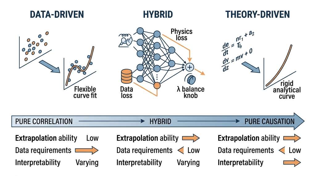
$$\hat{f} = \arg\min_{f \in \mathcal{F}} \underbrace{\sum_{i=1}^{N} \mathcal{L}(f(\mathbf{x}_i), y_i)}_{\text{data fidelity}} + \lambda \underbrace{\mathcal{R}_{\text{physics}}[f]}_{\text{theory constraint}}$$The physics regularizer \(\mathcal{R}_{\text{physics}}\) might penalize violations of a known conservation law, force the model to satisfy boundary conditions, or require consistency with a differential equation. The balance parameter \(\lambda\) controls how much the model trusts data versus theory. As shown in Figure 5.1, the three paradigms form a spectrum rather than isolated categories, with the hybrid approach occupying a tunable middle ground. Figure 5.1.1 illustrates the hybrid discovery spectrum from data-driven to theory-driven.
Checkpoint
So far: science progressed through four paradigms (empirical, theoretical, computational, data-intensive), and modern hybrid methods unify data-driven flexibility with theory-driven constraints via a single loss function whose balance parameter \(\lambda\) controls how much the model trusts observations versus physical laws.
Mental Model
Think of the balance parameter \(\lambda\) like seasoning a dish while following a recipe. The recipe (theory) tells you the correct proportions of ingredients, and your taste buds (data) tell you what actually tastes good. With \(\lambda = 0\) you ignore the recipe entirely and season by taste alone; the result may be delicious for this one meal but will not reproduce reliably. With \(\lambda \to \infty\) you follow the recipe to the letter regardless of how the dish tastes; if the recipe has an error, you are stuck. A well-chosen \(\lambda\) lets you follow the recipe's structure while adjusting to the actual ingredients in front of you. Just as a skilled cook trusts the recipe more for unfamiliar cuisines and their own palate more for dishes they know well, a hybrid model trusts theory more where data is sparse and data more where observations are dense.
The following example fits a curve with a physics-informed regularizer that enforces monotonicity, a physical constraint in many systems such as dose-response curves.
import numpy as np
from scipy.optimize import minimize

# Noisy observations of a monotonically increasing function
np.random.seed(21)
x_obs = np.sort(np.random.uniform(0, 5, 20))
y_true = 3.0 * (1 - np.exp(-0.8 * x_obs))  # saturating growth
y_obs = y_true + np.random.normal(0, 0.3, len(x_obs))

def model(x, params):
    """Flexible polynomial model: y = a0 + a1*x + a2*x^2 + a3*x^3"""
    return params[0] + params[1]*x + params[2]*x**2 + params[3]*x**3

def data_loss(params):
    return np.mean((model(x_obs, params) - y_obs)**2)

def monotonicity_penalty(params, n_check=100):
    """Penalize negative derivatives (enforce monotonicity)."""
    x_check = np.linspace(0, 5, n_check)
    # Derivative of polynomial: a1 + 2*a2*x + 3*a3*x^2
    deriv = params[1] + 2*params[2]*x_check + 3*params[3]*x_check**2
    violations = np.maximum(-deriv, 0)  # penalize negative slopes
    return np.mean(violations**2)

def hybrid_loss(params, lam=10.0):
    return data_loss(params) + lam * monotonicity_penalty(params)

# Pure data-driven fit (no constraint)
res_data = minimize(data_loss, x0=[0, 1, 0, 0], method='Nelder-Mead')

# Hybrid fit (data + monotonicity constraint)
res_hybrid = minimize(hybrid_loss, x0=[0, 1, 0, 0], method='Nelder-Mead')

x_plot = np.linspace(0, 5.5, 200)  # extend beyond data range
print("Data-only fit parameters:", np.round(res_data.x, 4))
print("Hybrid fit parameters:   ", np.round(res_hybrid.x, 4))

# Check: does data-only model violate monotonicity outside data range?
deriv_data = (res_data.x[1] + 2*res_data.x[2]*x_plot
              + 3*res_data.x[3]*x_plot**2)
violations = np.sum(deriv_data < 0)
print(f"Data-only model: {violations}/{len(x_plot)} points "
f"violate monotonicity")Data-only fit parameters: [-0.0637 1.5592 -0.2866 0.0152]
Hybrid fit parameters: [ 0.0422 1.1758 -0.1461 0.0042]
Data-only model: 11/200 points violate monotonicityThis small example previews a pattern that scales to the most sophisticated modern methods. Physics-informed neural networks (covered in depth in Chapter 33: Scientific Machine Learning) use exactly this architecture: a flexible neural network as \(\mathcal{F}\), data fidelity as one loss term, and PDE residuals as the physics regularizer.
Johannes Kepler spent eight years fitting ellipses to Tycho Brahe's observations of Mars, trying and discarding circular orbits, ovals, and egg shapes. His "Astronomia Nova" (1609) is arguably the first instance of data-driven model selection in science. He even computed what we would now call residuals, rejecting models whose errors exceeded 8 arcminutes, a threshold he considered unacceptable given Brahe's measurement precision of roughly 2 arcminutes. Modern Bayesian model selection formalizes exactly this process, as we will see in Chapter 32.
Step-Through: Hybrid Loss Evaluation
Trace through one iteration of the hybrid loss from Listing 5.3 with parameters \([a_0, a_1, a_2, a_3] = [0, 1.5, -0.3, 0.02]\) and \(\lambda = 10\).
Step 1 (Data loss): Evaluate the polynomial at each observed \(x_i\), compute squared errors, and average. Suppose the mean squared error over 20 points is \(\text{MSE} = 0.087\).
Step 2 (Derivative at check points): The derivative is \(a_1 + 2a_2 x + 3a_3 x^2 = 1.5 - 0.6x + 0.06x^2\). At \(x = 0\): derivative \(= 1.5\) (positive, no penalty). At \(x = 5\): derivative \(= 1.5 - 3.0 + 1.5 = 0.0\) (borderline, no penalty). At \(x = 6\): derivative \(= 1.5 - 3.6 + 2.16 = 0.06\) (still positive). This cubic barely stays monotone.
Step 3 (Monotonicity penalty): Since no check points have negative derivatives, \(\mathcal{R}_{\text{mono}} = 0\).
Step 4 (Hybrid loss): Total \(= 0.087 + 10 \times 0 = 0.087\). Now change \(a_3\) to \(-0.02\): at \(x = 5\) the derivative becomes \(1.5 - 3.0 + (-0.3) = -1.8\), yielding a large penalty \(\approx 1.62\), so the total loss jumps to \(0.087 + 10 \times 1.62 = 16.29\). The regularizer strongly steers the optimizer away from non-monotone solutions.
4. Comparing the Paradigms
Common Misconception
Readers often believe that data-driven and theory-driven discovery are competing alternatives, and that with enough data the theory-driven approach becomes obsolete. This is incorrect: data-driven models learn correlations within their training distribution, but they cannot reliably distinguish causal mechanisms from spurious associations (correlations that appear in the training data but do not reflect genuine cause-and-effect relationships), and they degrade unpredictably when extrapolating beyond observed conditions. Theory-driven models encode causal structure that generalizes by construction, which is why the two paradigms are complementary rather than substitutes.
The trade-offs summarized in Figure 5.1 also appear in the table below, with finer detail on each criterion. No single paradigm dominates; the art of discovery system design lies in choosing the right blend for the problem at hand.
| Criterion | Data-Driven | Theory-Driven | Hybrid |
|---|---|---|---|
| Data requirements | High (needs large N) | Low (needs parameters only) | Moderate |
| Domain knowledge | Optional | Essential | Leveraged |
| Extrapolation | Poor beyond training range | Strong if theory is correct | Improved over data-only |
| Interpretability | Varies (high for simple models) | High (equations have meaning) | Moderate |
| Flexibility | High | Low (rigid structure) | Tunable via \(\lambda\) |
| Discovery mode | Correlational patterns | Causal mechanisms | Constrained patterns |
The from-scratch polynomial fitting in Listings 5.1 and 5.3 takes about 30 lines. In production, sklearn.linear_model.LinearRegression handles the data-driven fit in 3 lines, while PySINDy automates the hybrid approach by discovering sparse governing equations from data using the SINDy (Sparse Identification of Nonlinear Dynamics) algorithm. PySINDy replaces the manual construction of physics regularizers with an automated sparse regression over a library of candidate terms, reducing hundreds of lines to about 10.
5. Implications for Discovery Systems
The trade-offs in that table are not merely academic; they surface as concrete architectural decisions every time you wire together a real discovery pipeline.
When you build a discovery system (the subject of Chapter 6), the choice between data-driven and theory-driven components is not made once. It is made at every module boundary. A system might use theory-driven simulation to generate training data, data-driven models to accelerate that simulation, and hybrid methods to validate whether the discovered patterns respect known physical laws.
The Discovery Workbench that we build throughout this book will need to support all three paradigms. Its surrogate modeling module (introduced in the next section) wraps expensive simulations in fast, uncertainty-aware approximations. Its active learning module, where the model selects its own training examples by choosing the experiments whose outcomes would most reduce its uncertainty, uses uncertainty to decide which experiment to run next. And its symbolic regression module (Chapter 35) attempts to distill learned models back into interpretable equations.
A rapidly developing direction uses large pretrained models as priors for scientific discovery. Instead of encoding domain knowledge as explicit equations, these approaches encode it as patterns learned from massive scientific corpora. Google DeepMind's GNoME system (2023) discovered 2.2 million stable crystal structures by combining graph neural networks with density functional theory calculations. More recently, Microsoft Research's Aurora model (2024) demonstrated that a single foundation model pretrained on over a million hours of diverse atmospheric simulation data can outperform state-of-the-art numerical weather prediction systems across forecasting, air quality estimation, and climate downscaling, all without task-specific retraining. Aurora exemplifies a shift from hand-crafted physics solvers to learned simulators that internalize physical constraints from data at scale, collapsing the boundary between "data-driven" and "theory-driven" into a unified learned representation. We explore this direction in Chapter 27: Scientific Foundation Models.
Try It: Data-Driven vs. Theory-Driven on Pendulum Data
Build and compare both paradigms on a single physical system using only Python, NumPy, and SciPy.
- Generate data. Simulate a simple pendulum using
scipy.integrate.solve_ivpwith the ODE \(\ddot{\theta} = -(g/L)\sin\theta\), setting \(g = 9.81\), \(L = 1.0\), and \(\theta_0 = 0.5\) rad. Record 100 time-angle pairs over 10 seconds and add Gaussian noise (\(\sigma = 0.02\)) to simulate measurement error. - Fit a data-driven model. Use
numpy.polyfitto fit a degree-8 polynomial to the noisy time-angle data. Plot the fit over the training interval and extrapolate 5 seconds beyond the data range. - Fit a theory-driven model. Using the known ODE, estimate the parameters \(g/L\) by minimizing the squared error between the ODE solution and the noisy data via
scipy.optimize.minimize. Plot this fit and its extrapolation over the same extended range. - Compare extrapolation. Generate ground-truth data for the full 15-second window. Compute the root-mean-square error (RMSE) of each model on the extrapolation interval (10 to 15 seconds). The polynomial will diverge; the ODE fit will track the true oscillation.
- Reflect. Write two sentences: under what condition would the data-driven model be preferable despite its extrapolation failure, and what would you need to add to make a hybrid version?
Exercise 5.1.1
You have two models for predicting the boiling point of organic molecules. Model A is a random forest trained on 10,000 measured boiling points. Model B solves the Clausius-Clapeyron equation using estimated enthalpies of vaporization. You need to predict boiling points for a novel class of fluorinated compounds absent from Model A's training set. Which model would you trust more for these out-of-distribution predictions, and why? What single piece of information would most change your answer?
Hint
Consider what "out-of-distribution" means for each paradigm. Model A learned statistical patterns from its training molecules; fluorinated compounds may have systematically different intermolecular forces. Model B encodes a thermodynamic relationship that holds regardless of molecular family, but its accuracy depends on the quality of the enthalpy estimates. The key information that could change your answer: does the training set for Model A already contain structurally similar halogenated compounds?
Real-World Application: Drug Discovery at Recursion Pharmaceuticals
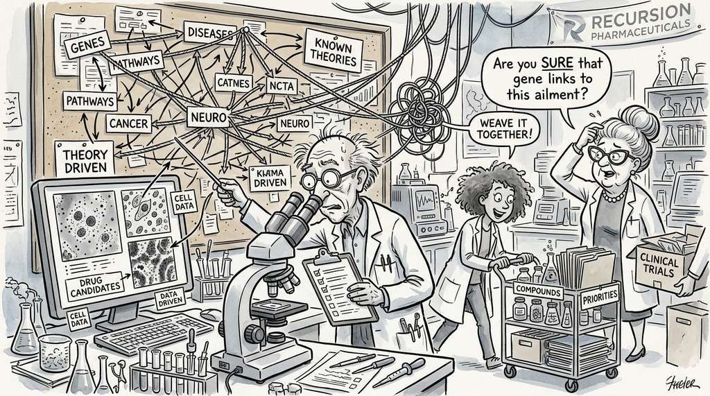
Recursion Pharmaceuticals uses a hybrid discovery pipeline in which high-content microscopy images of cells treated with drug candidates (data-driven) are combined with known gene-disease pathway maps (theory-driven) to prioritize compounds for clinical trials. Their system, which processes millions of cellular images per week, discovered that a compound originally developed for a rare genetic disease also showed efficacy against inflammatory bowel disease, a connection that pure theory or pure data alone had missed because it required both visual phenotypic patterns and mechanistic pathway reasoning.
Lab: Data vs. Theory on a Damped Oscillator
Goal: Experience firsthand how data-driven and theory-driven models diverge when extrapolating beyond training data.
Tools needed: Python 3, NumPy, SciPy (integrate.solve_ivp, optimize.curve_fit), Matplotlib. No GPU required; runs in under a minute on any laptop.
Procedure: (1) Simulate a damped harmonic oscillator (\(\ddot{x} + 2\zeta\omega_0 \dot{x} + \omega_0^2 x = 0\)) with \(\omega_0 = 2\pi\), \(\zeta = 0.1\), and \(x_0 = 1.0\) for 5 seconds. Record 200 noisy samples (\(\sigma = 0.05\)). (2) Fit a degree-12 polynomial to the first 3 seconds of data. (3) Fit the damped oscillator ODE to the same 3 seconds by optimizing \(\omega_0\) and \(\zeta\) via curve_fit. (4) Plot both models over the full 5 seconds alongside the ground truth.
What to vary: Try different noise levels (\(\sigma \in \{0.01, 0.05, 0.2\}\)) and different training windows (first 1, 2, or 3 seconds). Observe how the polynomial's extrapolation error grows explosively while the ODE fit remains stable.
What to observe: At what noise level does the ODE fit start to degrade? How does the length of the training window affect polynomial extrapolation? Record the ratio of extrapolation RMSE (polynomial vs. ODE) for each setting and note when, if ever, the polynomial wins.
Exercises
- Conceptual: A pharmaceutical company has 500 measured half-maximal inhibitory concentration (IC50) values for drug candidates against a single target. Would you recommend a data-driven, theory-driven, or hybrid model for predicting IC50 of new candidates? Justify your choice by considering data availability, the complexity of protein-ligand binding, and the need for extrapolation to novel chemical scaffolds.
- Coding: Modify Listing 5.3 to add a second physics constraint: the function must be concave (second derivative negative everywhere). Implement this as an additional penalty term and show that the hybrid model now fits a saturating curve that cannot "run away" at large \(x\).
- Analysis: Download the University of California, Irvine (UCI) "Concrete Compressive Strength" dataset. Fit three models: (a) a pure data-driven random forest, (b) Abrams' law (a theory-driven model relating strength to water-cement ratio), and (c) a hybrid that uses Abrams' law as a feature plus data-driven residual correction. Compare their test-set RMSE and discuss which model you would trust for a concrete mix far outside the training distribution.
What's Next
We have seen how data and theory each contribute to discovery. But what about the third pillar: simulation? In Section 5.2: Simulation and Surrogate Models, we explore how computational experiments create virtual laboratories, and how surrogate models make those experiments fast enough for real-time exploration. We will also confront a critical question: when your model makes a prediction, how much should you trust it?
Bibliography
The foundational collection that articulated data-intensive science as a fourth paradigm alongside experiment, theory, and simulation.
The paper that popularized PINNs, demonstrating how neural networks can learn solutions to PDEs while respecting physical constraints.
Introduced the SINDy algorithm for sparse equation discovery, bridging data-driven and theory-driven approaches with interpretable results.
Google DeepMind's GNoME system, which used graph neural networks to discover millions of stable crystal structures.
ESMFold: protein structure prediction from language models trained on evolutionary sequences, a data-driven approach encoding implicit physical knowledge. As of 2024, the successor model ESM3 (Hayes et al., 2024) extends this approach to jointly generate protein sequence, structure, and function.
Introduced Neural ODEs, which parameterize ODE dynamics with neural networks, enabling continuous-depth models and hybrid data-theory architectures.
A comprehensive survey of methods for incorporating physics into ML, covering soft constraints, architectural priors, and physics-informed losses.
The production library implementing SINDy and its extensions, with tutorials for equation discovery from time-series data.
AlphaFold's first breakthrough, demonstrating that data-driven deep learning could match physics-based methods for protein structure prediction. As of 2024, AlphaFold 2 (Jumper et al., 2021) and AlphaFold 3 (Abramson et al., 2024) have substantially surpassed this initial result, with AlphaFold 3 extending predictions to protein complexes, nucleic acids, and small-molecule ligands.
The standard Python library for data-driven modeling, providing regression, classification, and model selection tools used throughout this chapter.