45.1 Bayesian Optimization

1. The Black-Box Optimization Problem

A single neural architecture search can burn tens of thousands of GPU-hours if every candidate is evaluated from scratch. When each evaluation costs that much, choosing the wrong next experiment is not merely wasteful; it can exhaust the entire project budget before any useful result emerges. Bayesian optimization exists precisely for these high-stakes, low-budget regimes.

We seek to find the input \(\mathbf{x}^* \in \mathcal{X}\) that maximizes an unknown function \(f\):

where \(\mathcal{X} \subseteq \mathbb{R}^d\) is a bounded search space and \(f\) has no known closed form. Each evaluation \(y = f(\mathbf{x}) + \varepsilon\) is expensive, and noise \(\varepsilon \sim \mathcal{N}(0, \sigma^2_n)\) may corrupt the observation. We have no access to gradients \(\nabla f\). The budget \(N\) is small, typically 20 to a few hundred evaluations. Scientific discovery operates in exactly this regime: a lab can synthesize and test a modest number of compounds, run a limited set of simulations, or conduct a bounded number of physical experiments. In short: Bayesian optimization treats every expensive evaluation as precious, using a probabilistic surrogate to make each one count.

2. Gaussian Process Surrogates

A Gaussian process (GP) is a distribution over functions: any finite collection of function values \(\mathbf{f} = [f(\mathbf{x}_1), \ldots, f(\mathbf{x}_n)]^T\) follows a multivariate Gaussian distribution. A GP is fully specified by a mean function \(m(\mathbf{x})\) and a covariance (kernel) function \(k(\mathbf{x}, \mathbf{x}')\):

The kernel encodes our prior beliefs about \(f\): smoothness, periodicity, length scale, and amplitude. The most common choice is the Matérn 5/2 kernel:

where \(r = \sqrt{\sum_{i=1}^d \left(\frac{x_i - x'_i}{\ell_i}\right)^2}\) and \(\ell_i\) are per-dimension length scales. The Matérn 5/2 is twice differentiable (smoother than Matérn 3/2, less smooth than the squared-exponential), which tends to match the regularity of many physical and chemical response surfaces.

2.1 Posterior Inference

Given \(n\) observations \(\mathcal{D}_n = \{(\mathbf{x}_i, y_i)\}_{i=1}^n\), the GP posterior at a new point \(\mathbf{x}_*\) is also Gaussian with closed-form mean and variance:

where \(\mathbf{K}\) is the \(n \times n\) kernel matrix with entries \(K_{ij} = k(\mathbf{x}_i, \mathbf{x}_j)\), \(\mathbf{k}_*\) is the \(n\)-vector with entries \(k(\mathbf{x}_i, \mathbf{x}_*)\), and \(\mathbf{y} = [y_1, \ldots, y_n]^T\). The posterior mean \(\mu(\mathbf{x}_*)\) is our best estimate of \(f(\mathbf{x}_*)\); the posterior variance \(\sigma^2(\mathbf{x}_*)\) quantifies how uncertain we are. Points far from any observation have high variance; points near many observations have low variance.

The following class implements this from scratch, fitting a GP with a squared exponential kernel and predicting with calibrated uncertainties.

import numpy as np
from scipy.linalg import cho_solve, cho_factor
from scipy.optimize import minimize

class GaussianProcessRegressor:
    """Minimal GP regressor for Bayesian optimization.

    Uses the squared exponential kernel with per-dimension length scales
    and optimizes hyperparameters via marginal likelihood.
    """

    def __init__(self, noise: float = 1e-6):
        self.noise = noise
        self.length_scales = None
        self.signal_var = 1.0
        self.X_train = None
        self.y_train = None
        self._L = None  # Cholesky factor
        self._alpha = None  # Precomputed weights

    def _kernel(self, X1: np.ndarray, X2: np.ndarray) -> np.ndarray:
        """Squared exponential kernel with ARD length scales."""
        X1_scaled = X1 / self.length_scales
        X2_scaled = X2 / self.length_scales
        sq_dists = (
            np.sum(X1_scaled**2, axis=1, keepdims=True)
            + np.sum(X2_scaled**2, axis=1)
            - 2 * X1_scaled @ X2_scaled.T
        )
        return self.signal_var * np.exp(-0.5 * sq_dists)

    def _neg_log_marginal_likelihood(self, theta: np.ndarray) -> float:
        """Negative log marginal likelihood for hyperparameter optimization."""
        d = self.X_train.shape[1]
        self.length_scales = np.exp(theta[:d])
        self.signal_var = np.exp(theta[d])

        K = self._kernel(self.X_train, self.X_train)
        K += self.noise * np.eye(len(K))

        try:
            L = cho_factor(K)
            alpha = cho_solve(L, self.y_train)
            # log p(y|X,theta) = -0.5 * y^T alpha - sum(log(diag(L))) - n/2 log(2pi)
            nll = (
                0.5 * self.y_train @ alpha
                + np.sum(np.log(np.diag(L[0])))
                + 0.5 * len(self.y_train) * np.log(2 * np.pi)
            )
            return nll
        except np.linalg.LinAlgError:
            return 1e10  # Return large value for non-PD matrices

    def fit(self, X: np.ndarray, y: np.ndarray) -> "GaussianProcessRegressor":
        """Fit the GP by optimizing kernel hyperparameters."""
        self.X_train = np.asarray(X, dtype=np.float64)
        self.y_train = np.asarray(y, dtype=np.float64)
        d = X.shape[1]

        # Initialize length scales to data range, signal variance to data variance
        self.length_scales = np.ones(d)
        theta0 = np.zeros(d + 1)  # log length scales + log signal variance

        result = minimize(
            self._neg_log_marginal_likelihood,
            theta0,
            method="L-BFGS-B",
            bounds=[(-3, 3)] * (d + 1),
        )
        self.length_scales = np.exp(result.x[:d])
        self.signal_var = np.exp(result.x[d])

        # Precompute for prediction
        K = self._kernel(self.X_train, self.X_train)
        K += self.noise * np.eye(len(K))
        self._L = cho_factor(K)
        self._alpha = cho_solve(self._L, self.y_train)
        return self

    def predict(self, X: np.ndarray) -> tuple:
        """Return posterior mean and standard deviation."""
        X = np.asarray(X, dtype=np.float64)
        K_star = self._kernel(X, self.X_train)
        mu = K_star @ self._alpha

        v = cho_solve(self._L, K_star.T)
        var = self.signal_var - np.sum(K_star.T * v, axis=0)
        var = np.maximum(var, 1e-10)  # Numerical floor
        return mu, np.sqrt(var)

3. Acquisition Functions

The GP posterior gives us a belief about \(f\) everywhere in \(\mathcal{X}\). The acquisition function \(\alpha(\mathbf{x})\) converts this belief into a scalar score that quantifies the "utility" of evaluating \(f\) at \(\mathbf{x}\). We maximize the acquisition function (which is cheap, since it uses only the GP posterior) to select the next evaluation point:

Three acquisition functions dominate practice:

3.1 Probability of Improvement (PI)

Let \(f^+ = \max_{i=1}^n y_i\) be the best observed value. PI measures the probability that the new point exceeds \(f^+\):

where \(\Phi\) is the standard normal CDF and \(\xi \geq 0\) is a small "jitter" that prevents pure exploitation. PI is simple but greedy: it weights a tiny improvement the same as a massive one.

3.2 Expected Improvement (EI)

The EI formula balances exploration and exploitation without a tuning parameter, making it the default choice in most BO implementations. (This is a key reason EI is often preferred over UCB in practice: UCB requires tuning \(\beta_t\) per problem, while EI delivers a principled explore/exploit balance out of the box.) The implementation follows:

from scipy.stats import norm

def expected_improvement(
    X_candidates: np.ndarray,
    gp: GaussianProcessRegressor,
    y_best: float,
    xi: float = 0.01,
) -> np.ndarray:
    """Compute Expected Improvement at candidate points.

    Parameters
    ----------
    X_candidates : array of shape (m, d)
        Points at which to evaluate the acquisition function.
    gp : GaussianProcessRegressor
        Fitted GP surrogate.
    y_best : float
        Best observed value so far.
    xi : float
        Exploration-exploitation trade-off parameter (small positive).

    Returns
    -------
    ei : array of shape (m,)
        Expected improvement values.
    """
    mu, sigma = gp.predict(X_candidates)

    with np.errstate(divide="ignore", invalid="ignore"):
        improvement = mu - y_best - xi
        Z = improvement / sigma
        ei = improvement * norm.cdf(Z) + sigma * norm.pdf(Z)
        ei[sigma < 1e-10] = 0.0  # No improvement where GP is certain

    return ei

3.3 Upper Confidence Bound (UCB)

The GP-UCB acquisition function adds a scaled uncertainty bonus to the posterior mean:

where \(\beta_t\) controls the exploration-exploitation balance and can be set to achieve sublinear regret bounds. Srinivas et al. (2010) proved that \(\beta_t = 2 \log(|\mathcal{X}| t^2 \pi^2 / 6\delta)\) yields cumulative regret (the total shortfall between the values chosen and the true optimum) of \(O(\sqrt{T \gamma_T \log T})\), where \(\gamma_T\) is the maximum information gain (a measure of how much the GP can learn about \(f\) from \(T\) observations, determined by the kernel's eigenvalue decay). In practice, \(\beta_t\) between 1 and 3 works well. This connects directly to the UCB strategy from Section 1.2, but now applied to continuous spaces via the GP posterior.

4. The Bayesian Optimization Loop

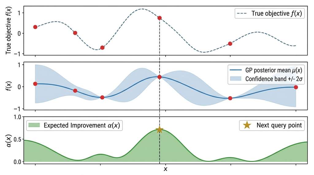
These two components, the GP surrogate and the acquisition function, combine into a single iterative algorithm. The loop is illustrated in Figure 45.1.

The complete BO algorithm iterates three steps: (1) fit the GP to all observations, (2) maximize the acquisition function to select the next query point, and (3) evaluate the expensive objective at that point. The loop begins with a Latin hypercube initialization (a space-filling sampling scheme that divides each dimension into equal-probability intervals, ensuring initial points cover the search space more uniformly than purely random sampling). Here is a from-scratch implementation: Figure 45.1.1 illustrates Bayesian optimization loop with GP surrogate and acquisition function.

from typing import Callable

def bayesian_optimization(
    objective: Callable,
    bounds: np.ndarray,
    n_init: int = 5,
    n_iter: int = 25,
    seed: int = 42,
) -> dict:
    """Run Bayesian optimization on a black-box objective.

    Parameters
    ----------
    objective : callable
        Function f(x) -> float to maximize. x is a 1-D array.
    bounds : array of shape (d, 2)
        Lower and upper bounds for each dimension.
    n_init : int
        Number of initial random evaluations (Latin hypercube).
    n_iter : int
        Number of BO iterations after initialization.
    seed : int
        Random seed.

    Returns
    -------
    dict with keys 'X' (all evaluated points), 'y' (all values),
    'best_x', 'best_y', 'history' (best value at each step).
    """
    rng = np.random.default_rng(seed)
    d = bounds.shape[0]

    # Latin hypercube initialization
    X = rng.uniform(bounds[:, 0], bounds[:, 1], size=(n_init, d))
    y = np.array([objective(x) for x in X])

    history = [np.max(y)]
    gp = GaussianProcessRegressor(noise=1e-4)

    for i in range(n_iter):
        # Step 1: Fit GP to all observations
        gp.fit(X, y)

        # Step 2: Maximize acquisition function via random + local search
        n_candidates = 5000
        X_cand = rng.uniform(bounds[:, 0], bounds[:, 1], size=(n_candidates, d))
        ei = expected_improvement(X_cand, gp, y_best=np.max(y))

        # Refine top candidates with L-BFGS-B
        top_k = X_cand[np.argsort(ei)[-5:]]
        best_ei, best_x = -1, None
        for x0 in top_k:
            result = minimize(
                lambda x: -expected_improvement(x.reshape(1, -1), gp, np.max(y))[0],
                x0,
                bounds=list(zip(bounds[:, 0], bounds[:, 1])),
                method="L-BFGS-B",
            )
            if -result.fun > best_ei:
                best_ei = -result.fun
                best_x = result.x

        # Step 3: Evaluate the expensive objective
        y_new = objective(best_x)
        X = np.vstack([X, best_x.reshape(1, -1)])
        y = np.append(y, y_new)
        history.append(np.max(y))

    best_idx = np.argmax(y)
    return {
        "X": X, "y": y,
        "best_x": X[best_idx], "best_y": y[best_idx],
        "history": history,
    }

5. Practical BO with BoTorch

The from-scratch implementation above clarifies the mechanics, but production BO uses libraries that handle numerical stability, GPU acceleration, batch acquisition, and multi-output GPs. BoTorch, built on PyTorch and GPyTorch, is the standard for research-grade Bayesian optimization.

import torch
from botorch.models import SingleTaskGP
from botorch.fit import fit_gpytorch_mll
from botorch.acquisition import ExpectedImprovement
from botorch.optim import optimize_acqf
from gpytorch.mlls import ExactMarginalLogLikelihood

def botorch_bo_step(
    train_X: torch.Tensor,
    train_Y: torch.Tensor,
    bounds: torch.Tensor,
) -> torch.Tensor:
    """One step of BO using BoTorch: fit GP, optimize EI, return next point.

    Parameters
    ----------
    train_X : Tensor of shape (n, d)
        Observed inputs, scaled to [0, 1]^d.
    train_Y : Tensor of shape (n, 1)
        Observed outputs, standardized.
    bounds : Tensor of shape (2, d)
        Lower and upper bounds (typically 0 and 1).

    Returns
    -------
    next_x : Tensor of shape (1, d)
        The next point to evaluate.
    """
    # Fit a GP with automatic hyperparameter tuning
    gp = SingleTaskGP(train_X, train_Y)
    mll = ExactMarginalLogLikelihood(gp.likelihood, gp)
    fit_gpytorch_mll(mll)

    # Construct and optimize the EI acquisition function
    best_f = train_Y.max()
    ei = ExpectedImprovement(model=gp, best_f=best_f)

    next_x, acq_value = optimize_acqf(
        acq_function=ei,
        bounds=bounds,
        q=1,            # Single-point acquisition
        num_restarts=10,
        raw_samples=512,
    )
    return next_x

import optuna

def objective(trial):
    x1 = trial.suggest_float("x1", 0.0, 1.0)
    x2 = trial.suggest_float("x2", 0.0, 1.0)
    return expensive_function(x1, x2)

study = optuna.create_study(
    direction="maximize",
    sampler=optuna.samplers.TPESampler(seed=42),
)
study.optimize(objective, n_trials=30)

print(f"Best: {study.best_value:.4f} at {study.best_params}")

6. Batch Bayesian Optimization

The methods above select one evaluation at a time, but many real laboratories and compute clusters can run several experiments simultaneously.

When you can run experiments in parallel (multiple synthesis stations, a GPU cluster), you want to select a batch of \(q\) points simultaneously. Naive parallelization (selecting the top \(q\) EI points independently) fails because those points will cluster near the same optimum. Batch BO methods account for the correlations between pending evaluations.

The \(q\)-Expected Improvement (\(q\)-EI) acquisition function jointly optimizes over \(q\) candidate points:

This integral has no closed form for \(q > 1\), but BoTorch computes it efficiently via Monte Carlo sampling from the GP posterior:

from botorch.acquisition import qExpectedImprovement

def batch_bo_step(
    train_X: torch.Tensor,
    train_Y: torch.Tensor,
    bounds: torch.Tensor,
    batch_size: int = 4,
) -> torch.Tensor:
    """Select a batch of points for parallel evaluation."""
    gp = SingleTaskGP(train_X, train_Y)
    mll = ExactMarginalLogLikelihood(gp.likelihood, gp)
    fit_gpytorch_mll(mll)

    qei = qExpectedImprovement(
        model=gp,
        best_f=train_Y.max(),
        sampler=torch.quasirandom.SobolEngine(dimension=1),
    )

    candidates, _ = optimize_acqf(
        acq_function=qei,
        bounds=bounds,
        q=batch_size,
        num_restarts=10,
        raw_samples=512,
    )
    return candidates  # Shape: (batch_size, d)

7. When Bayesian Optimization Struggles

Batch acquisition broadens the practical reach of BO, yet even with parallelism the method carries fundamental assumptions about smoothness, dimensionality, and evaluation cost that do not always hold.

BO is not universally optimal. Its limitations define the boundaries of its applicability and motivate the evolutionary and RL methods in the following sections:

• High dimensionality (\(d > 20\)): GP kernel matrices grow as \(O(n^3)\) and the acquisition landscape becomes increasingly multimodal. Random Embedding Bayesian Optimization (REMBO) and Trust Region Bayesian Optimization (TuRBO) partially address this, but evolutionary methods scale more naturally.
• Combinatorial or discrete spaces: GPs assume continuous inputs. Categorical variables require specialized kernels or embeddings.
• Many objectives (\(m > 3\)): Multi-objective BO exists (Section 45.4 uses it), but the Pareto front (the set of solutions where no objective can be improved without worsening another) becomes exponentially harder to approximate. Non-dominated Sorting Genetic Algorithm III (NSGA-III) handles many objectives more gracefully.
• Non-stationary objectives: Standard kernels assume the function's smoothness is uniform across the space. If roughness varies spatially, deep kernel learning or input warping is needed.
• Very large evaluation budgets (\(N > 1000\)): When evaluations are cheap enough to run thousands of them, the GP overhead outweighs the sample-efficiency gain. Evolutionary methods or random search with early stopping become competitive.

8. Discovery Workbench Integration

The Discovery Workbench (introduced in Chapter 6) gains a BayesianOptimizer component that wraps the BO loop above. The optimizer accepts any objective function registered through the Workbench's experiment runner. It logs all evaluations, GP hyperparameters, and acquisition function values to the experiment registry (Chapter 47). These logs enable retrospective analysis of the optimization trajectory: which regions did the GP explore? Where did EI disagree with the final optimum? Did the length-scale estimates converge?

from discovery_workbench import Optimizer, ExperimentRegistry

class WorkbenchBayesianOptimizer(Optimizer):
    """BO optimizer integrated with the Discovery Workbench."""

    def __init__(self, bounds, registry: ExperimentRegistry, **kwargs):
        self.bounds = torch.tensor(bounds, dtype=torch.float64)
        self.registry = registry
        self.train_X = torch.empty(0, len(bounds))
        self.train_Y = torch.empty(0, 1)

    def suggest(self, n_suggestions: int = 1) -> list:
        """Suggest next experiment(s) to run."""
        if len(self.train_X) < 5:
            # Random initialization phase
            candidates = torch.rand(n_suggestions, self.bounds.shape[0])
            candidates = self.bounds[0] + candidates * (self.bounds[1] - self.bounds[0])
        else:
            candidates = batch_bo_step(
                self.train_X, self.train_Y, self.bounds, batch_size=n_suggestions
            )

        # Log suggestions to the experiment registry
        self.registry.log_suggestions(candidates.numpy(), method="bayesian_optimization")
        return candidates.numpy().tolist()

    def observe(self, X, y):
        """Record experiment results."""
        X_new = torch.tensor(X, dtype=torch.float64).reshape(-1, self.bounds.shape[0])
        y_new = torch.tensor(y, dtype=torch.float64).reshape(-1, 1)
        self.train_X = torch.cat([self.train_X, X_new])
        self.train_Y = torch.cat([self.train_Y, y_new])
        self.registry.log_observations(X_new.numpy(), y_new.numpy())