22.1 Model Lifecycle Management

The Big Picture

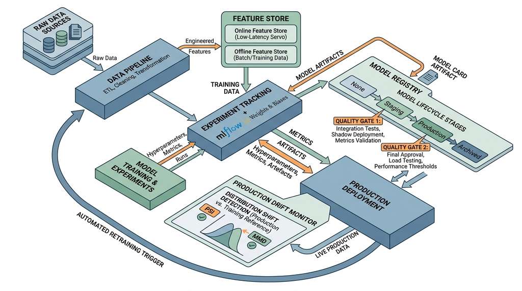
When a pharmaceutical company's drug activity predictor silently began returning wrong scores for an entire compound class, the root cause turned out to be a single renamed column in an upstream CSV, changed six weeks earlier, with no record of the modification anywhere in the pipeline. That failure captures the central problem: a model in production is not a static artifact but a living system embedded in data transformations, feature computations, training runs, evaluation gates, deployment stages, and monitoring loops. Model lifecycle management is the discipline of making every step in this pipeline reproducible, auditable, and automated. Without it, you get "works on my laptop" science: models that cannot be retrained, results that cannot be reproduced, and production failures that cannot be diagnosed. This section builds the operational backbone that the rest of the chapter depends on. Figure 22.1.1 illustrates the ML model lifecycle pipeline.

1. Data Pipelines and Feature Stores

When a regulatory auditor asks which data produced last quarter's predictions, or a retrained model silently degrades because an upstream CSV column was renamed, the absence of a formal pipeline turns a routine question into a crisis. The discipline described next exists to prevent exactly that scenario.

Every machine learning (ML) system begins with data, and every production failure eventually traces back to data. A data pipeline is a directed acyclic graph (DAG) of transformations that converts raw data sources into training-ready datasets. The critical properties are reproducibility (the same inputs produce the same outputs), idempotency (where re-running a step on the same inputs produces the same result without corrupting or duplicating state), and observability (you can inspect every intermediate result).

A data pipeline matters because without one, every model retraining becomes a manual, error-prone process. A single missed transformation silently corrupts results. Each stage in the DAG declares its inputs (files, parameters, upstream stage outputs) and its outputs. The orchestrator hashes all inputs to decide whether a stage needs re-execution or can serve cached results. Use a formal pipeline (DVC, Airflow, Prefect) rather than ad hoc scripts whenever your workflow has more than one transformation step, multiple contributors, or any requirement for auditability. (DVC is introduced briefly here for its pipeline capabilities; Section 5 below covers its data versioning features in depth.) Reserve bare scripts for throwaway explorations that will never reach production.

The simplest data pipeline is a Python script that reads a CSV, applies transformations, and writes a parquet file. The problem is that this script carries no metadata: when was it run, on what input, with which library versions, and what did the output look like? A proper pipeline tool adds this metadata automatically. In short: if your pipeline carries no metadata, your model carries no provenance.

"""
A minimal data pipeline using DVC (Data Version Control).
DVC tracks data files alongside code in Git, enabling
reproducible pipelines without storing large files in the repo.
"""
import pandas as pd
import numpy as np
from pathlib import Path
import json
import hashlib

class DataPipeline:
    """Reproducible data pipeline with lineage tracking."""

    def __init__(self, raw_dir: str, processed_dir: str):
        self.raw_dir = Path(raw_dir)
        self.processed_dir = Path(processed_dir)
        self.processed_dir.mkdir(parents=True, exist_ok=True)
        self.lineage = {
            "steps": [],
            "input_hashes": {},
            "output_hashes": {}
        }

    def _hash_file(self, path: Path) -> str:
        """Compute SHA-256 hash for data lineage tracking."""
        h = hashlib.sha256()
        with open(path, "rb") as f:
            for chunk in iter(lambda: f.read(8192), b""):
                h.update(chunk)
        return h.hexdigest()

    def ingest(self, filename: str) -> pd.DataFrame:
        """Load raw data and record its hash for provenance."""
        path = self.raw_dir / filename
        df = pd.read_csv(path)
        self.lineage["input_hashes"][filename] = self._hash_file(path)
        self.lineage["steps"].append({
            "action": "ingest",
            "file": filename,
            "rows": len(df),
            "columns": list(df.columns)
        })
        return df

    def validate(self, df: pd.DataFrame, schema: dict) -> pd.DataFrame:
        """Validate data against expected schema and ranges."""
        errors = []
        for col, rules in schema.items():
            if col not in df.columns:
                errors.append(f"Missing column: {col}")
                continue
            if "dtype" in rules:
                if not pd.api.types.is_dtype_equal(df[col].dtype, rules["dtype"]):
                    df[col] = df[col].astype(rules["dtype"])
            if "min" in rules and df[col].min() < rules["min"]:
                errors.append(f"{col}: min {df[col].min()} < {rules['min']}")
            if "max" in rules and df[col].max() > rules["max"]:
                errors.append(f"{col}: max {df[col].max()} > {rules['max']}")
            if "nullable" in rules and not rules["nullable"]:
                null_count = df[col].isnull().sum()
                if null_count > 0:
                    errors.append(f"{col}: {null_count} null values")

        self.lineage["steps"].append({
            "action": "validate",
            "errors": errors,
            "passed": len(errors) == 0
        })
        if errors:
            raise ValueError(f"Validation failed: {errors}")
        return df

    def transform(self, df: pd.DataFrame,
                  transformations: list[dict]) -> pd.DataFrame:
        """Apply a sequence of named transformations."""
        for t in transformations:
            if t["type"] == "log_transform":
                col = t["column"]
                df[f"{col}_log"] = np.log1p(df[col])
            elif t["type"] == "normalize":
                col = t["column"]
                mean, std = df[col].mean(), df[col].std()
                df[f"{col}_norm"] = (df[col] - mean) / std
                # Store parameters for serving-time consistency
                t["params"] = {"mean": float(mean), "std": float(std)}
            elif t["type"] == "one_hot":
                col = t["column"]
                dummies = pd.get_dummies(df[col], prefix=col)
                df = pd.concat([df, dummies], axis=1)

        self.lineage["steps"].append({
            "action": "transform",
            "transformations": transformations,
            "output_shape": list(df.shape)
        })
        return df

    def save(self, df: pd.DataFrame, filename: str) -> Path:
        """Save processed data and record output hash."""
        path = self.processed_dir / filename
        df.to_parquet(path, index=False)
        self.lineage["output_hashes"][filename] = self._hash_file(path)

        # Save lineage metadata alongside the data
        lineage_path = path.with_suffix(".lineage.json")
        with open(lineage_path, "w") as f:
            json.dump(self.lineage, f, indent=2, default=str)

        return path


# Usage: a reproducible pipeline run
pipeline = DataPipeline("data/raw", "data/processed")
df = pipeline.ingest("molecules.csv")
df = pipeline.validate(df, {
    "molecular_weight": {"dtype": "float64", "min": 0, "max": 2000},
    "logp": {"dtype": "float64", "min": -10, "max": 20},
    "activity": {"dtype": "float64", "nullable": False}
})
df = pipeline.transform(df, [
    {"type": "log_transform", "column": "molecular_weight"},
    {"type": "normalize", "column": "logp"}
])
pipeline.save(df, "molecules_processed.parquet")

The pipeline above handles the mechanics, but production systems also need a feature store: a centralized repository of computed features that decouples feature engineering from model training. A feature store serves two purposes. First, it ensures that the same feature computation runs at training time and serving time, preventing the notorious training-serving skew where features are computed differently in batch training and online inference. Second, it enables feature reuse: a "molecular_weight_log" feature computed once can be shared across dozens of models without recomputation.

"""
A minimal feature store implementation.
Production systems use Feast, Tecton, or Hopsworks; this shows
the core abstraction: named features with versioned definitions.
"""
from dataclasses import dataclass, field
from datetime import datetime
from typing import Callable
import pandas as pd

@dataclass
class FeatureDefinition:
    """A versioned, named feature with its computation function."""
    name: str
    version: int
    description: str
    dtype: str
    compute_fn: Callable[[pd.DataFrame], pd.Series]
    created_at: datetime = field(default_factory=datetime.now)
    dependencies: list[str] = field(default_factory=list)

class FeatureStore:
    """In-memory feature store with versioning and lineage."""

    def __init__(self):
        self._registry: dict[str, FeatureDefinition] = {}
        self._cache: dict[str, pd.Series] = {}

    def register(self, feature: FeatureDefinition) -> None:
        """Register a feature definition. Newer versions overwrite."""
        key = f"{feature.name}_v{feature.version}"
        self._registry[key] = feature
        # Also store as "latest"
        self._registry[feature.name] = feature

    def compute(self, name: str, df: pd.DataFrame,
                version: int | None = None) -> pd.Series:
        """Compute a feature, using cache if available."""
        key = f"{name}_v{version}" if version else name
        if key not in self._registry:
            raise KeyError(f"Feature '{key}' not registered")

        feature_def = self._registry[key]

        # Resolve dependencies first
        for dep in feature_def.dependencies:
            if dep not in df.columns:
                df[dep] = self.compute(dep, df)

        cache_key = f"{key}_{id(df)}"
        if cache_key not in self._cache:
            self._cache[cache_key] = feature_def.compute_fn(df)
        return self._cache[cache_key]

    def get_training_set(self, feature_names: list[str],
                         df: pd.DataFrame) -> pd.DataFrame:
        """Compute multiple features into a training DataFrame."""
        result = pd.DataFrame()
        for name in feature_names:
            result[name] = self.compute(name, df)
        return result


# Register features with explicit version and computation
store = FeatureStore()
store.register(FeatureDefinition(
    name="mol_weight_log",
    version=1,
    description="Log-transformed molecular weight",
    dtype="float64",
    compute_fn=lambda df: np.log1p(df["molecular_weight"])
))
store.register(FeatureDefinition(
    name="lipophilicity_normalized",
    version=1,
    description="Z-score normalized logP",
    dtype="float64",
    compute_fn=lambda df: (df["logp"] - df["logp"].mean()) / df["logp"].std()
))

With data pipelines producing versioned datasets and feature stores ensuring consistent feature computation, the next challenge is tracking the experiments that consume those features: which model architectures, hyperparameters, and training strategies actually produce good results.

2. Experiment Tracking

Model development is inherently experimental: different architectures, hyperparameters, feature sets, and training strategies compete, and only metrics reveal what works. Without systematic tracking, this process degenerates into scattered Jupyter notebooks and folders named "final_v3_ACTUALLY_FINAL." Experiment tracking tools record every run's parameters, metrics, artifacts, and code version in a searchable database.

MLflow is the most widely adopted open-source experiment tracking platform. Its Tracking component logs parameters, metrics, and artifacts for every training run. Its Model Registry manages model versions and lifecycle stages (Staging, Production, Archived). And its Projects component packages code for reproducible execution.

"""
Experiment tracking with MLflow: logging parameters, metrics,
artifacts, and registering the model for lifecycle management.
"""
import mlflow
import mlflow.sklearn
from sklearn.ensemble import RandomForestClassifier
from sklearn.model_selection import cross_val_score
from sklearn.metrics import (
    accuracy_score, precision_score, recall_score, f1_score,
    roc_auc_score, confusion_matrix
)
import numpy as np
import json

def train_and_track(
    X_train, y_train, X_test, y_test,
    experiment_name: str = "molecule_activity_prediction",
    params: dict | None = None
) -> str:
    """Train a model with full MLflow lifecycle tracking."""

    # Set or create the experiment
    mlflow.set_experiment(experiment_name)

    # Default hyperparameters
    params = params or {
        "n_estimators": 100,
        "max_depth": 10,
        "min_samples_split": 5,
        "min_samples_leaf": 2,
        "class_weight": "balanced"
    }

    with mlflow.start_run() as run:
        # 1. Log all hyperparameters
        mlflow.log_params(params)
        mlflow.log_param("n_features", X_train.shape[1])
        mlflow.log_param("n_samples_train", X_train.shape[0])
        mlflow.log_param("n_samples_test", X_test.shape[0])

        # 2. Train the model
        model = RandomForestClassifier(**params, random_state=42)
        model.fit(X_train, y_train)

        # 3. Evaluate and log metrics
        y_pred = model.predict(X_test)
        y_prob = model.predict_proba(X_test)[:, 1]

        metrics = {
            "accuracy": accuracy_score(y_test, y_pred),
            "precision": precision_score(y_test, y_pred),
            "recall": recall_score(y_test, y_pred),
            "f1": f1_score(y_test, y_pred),
            "roc_auc": roc_auc_score(y_test, y_prob)
        }
        mlflow.log_metrics(metrics)

        # 4. Log cross-validation scores for stability assessment
        cv_scores = cross_val_score(model, X_train, y_train, cv=5)
        mlflow.log_metric("cv_mean", cv_scores.mean())
        mlflow.log_metric("cv_std", cv_scores.std())

        # 5. Log feature importances as an artifact
        importance = dict(zip(
            [f"feature_{i}" for i in range(X_train.shape[1])],
            model.feature_importances_.tolist()
        ))
        with open("feature_importance.json", "w") as f:
            json.dump(importance, f, indent=2)
        mlflow.log_artifact("feature_importance.json")

        # 6. Log the confusion matrix
        cm = confusion_matrix(y_test, y_pred).tolist()
        mlflow.log_dict({"confusion_matrix": cm}, "confusion_matrix.json")

        # 7. Log the model itself with signature
        from mlflow.models import infer_signature
        signature = infer_signature(X_test, y_pred)
        mlflow.sklearn.log_model(
            model, "model",
            signature=signature,
            registered_model_name="molecule_activity_classifier"
        )

        print(f"Run ID: {run.info.run_id}")
        print(f"Metrics: {metrics}")
        return run.info.run_id

Weights & Biases (W&B) offers a complementary approach with richer visualization, collaborative features, and built-in hyperparameter sweep orchestration. The core abstraction is the same (runs with parameters, metrics, and artifacts), but W&B adds interactive dashboards, model comparison tables, and artifact lineage graphs that make experiment analysis more visual and collaborative.

"""
Experiment tracking with Weights & Biases, showing the
same workflow with W&B's richer API for sweeps and artifacts.
"""
import wandb
from sklearn.ensemble import GradientBoostingClassifier
from sklearn.metrics import f1_score, roc_auc_score

def train_with_wandb(X_train, y_train, X_test, y_test, config=None):
    """Train with W&B tracking, including artifact versioning."""

    # Initialize a W&B run
    run = wandb.init(
        project="molecule-activity",
        config=config or {
            "model": "gradient_boosting",
            "n_estimators": 200,
            "learning_rate": 0.1,
            "max_depth": 5,
            "subsample": 0.8
        }
    )
    config = wandb.config  # Access resolved config

    # Train the model
    model = GradientBoostingClassifier(
        n_estimators=config.n_estimators,
        learning_rate=config.learning_rate,
        max_depth=config.max_depth,
        subsample=config.subsample,
        random_state=42
    )
    model.fit(X_train, y_train)

    # Log metrics at each boosting stage for learning curves
    for i, y_pred_staged in enumerate(model.staged_predict(X_test)):
        wandb.log({
            "stage": i,
            "f1": f1_score(y_test, y_pred_staged),
        })

    # Final metrics
    y_pred = model.predict(X_test)
    y_prob = model.predict_proba(X_test)[:, 1]
    wandb.log({
        "final_f1": f1_score(y_test, y_pred),
        "final_roc_auc": roc_auc_score(y_test, y_prob),
    })

    # Log the model as a versioned artifact
    artifact = wandb.Artifact(
        "molecule-classifier", type="model",
        description="Gradient boosting classifier for molecular activity"
    )
    artifact.add_file("model.pkl")  # Would serialize model here
    run.log_artifact(artifact)

    run.finish()


# W&B Sweep: automated hyperparameter search
sweep_config = {
    "method": "bayes",  # Bayesian optimization
    "metric": {"name": "final_f1", "goal": "maximize"},
    "parameters": {
        "n_estimators": {"values": [100, 200, 500]},
        "learning_rate": {"distribution": "log_uniform_values",
                          "min": 0.001, "max": 0.3},
        "max_depth": {"values": [3, 5, 7, 10]},
        "subsample": {"distribution": "uniform",
                      "min": 0.6, "max": 1.0}
    }
}
# sweep_id = wandb.sweep(sweep_config, project="molecule-activity")
# wandb.agent(sweep_id, train_with_wandb, count=20)

3. Model Registry and Lifecycle Stages

An experiment tracker tells you which model is best. A model registry tells you which model is in production. The registry is a versioned catalog of trained models, each annotated with metadata (who trained it, on what data, with what performance) and a lifecycle stage that governs deployment decisions. Figure 22.1 illustrates the four stages and the quality gates (automated checks that a model must pass before advancing to the next stage) that govern transitions between them.

MLflow's Model Registry defines four stages: None (just logged), Staging (promoted for testing), Production (serving live traffic), and Archived (retired). Transitions between stages can be gated by automated checks: a model moves to Staging only if its test metrics exceed thresholds, and to Production only after passing integration tests and approval review. MLflow 2.9 (late 2023) deprecates these string-based stages in favor of model version aliases and tags, which allow more flexible promotion workflows. The stage-based API shown below still functions, but new projects should prefer the aliases API.

"""
Model registry operations: promoting models through lifecycle
stages with automated quality gates.
"""
from mlflow.tracking import MlflowClient
from dataclasses import dataclass

@dataclass
class QualityGate:
    """A metric threshold that must be met for stage promotion."""
    metric: str
    threshold: float
    comparison: str = "gte"  # "gte" or "lte"

    def passes(self, value: float) -> bool:
        if self.comparison == "gte":
            return value >= self.threshold
        return value <= self.threshold

class ModelLifecycleManager:
    """Manage model promotion through lifecycle stages."""

    def __init__(self, model_name: str):
        self.client = MlflowClient()
        self.model_name = model_name

    def get_latest_version(self, stage: str = "None") -> dict:
        """Get the latest model version in a given stage."""
        versions = self.client.get_latest_versions(
            self.model_name, stages=[stage]
        )
        if not versions:
            raise ValueError(
                f"No versions in stage '{stage}' for {self.model_name}"
            )
        return versions[0]

    def promote_to_staging(
        self, run_id: str, gates: list[QualityGate]
    ) -> bool:
        """Promote a run's model to Staging if it passes quality gates."""
        run = self.client.get_run(run_id)
        metrics = run.data.metrics

        # Check all quality gates
        failures = []
        for gate in gates:
            value = metrics.get(gate.metric)
            if value is None:
                failures.append(f"Missing metric: {gate.metric}")
            elif not gate.passes(value):
                failures.append(
                    f"{gate.metric}={value:.4f} "
                    f"failed threshold {gate.threshold}"
                )

        if failures:
            print(f"Promotion blocked: {failures}")
            return False

        # Find the model version from this run
        versions = self.client.search_model_versions(
            f"run_id='{run_id}'"
        )
        if versions:
            version = versions[0].version
            self.client.transition_model_version_stage(
                self.model_name, version, "Staging"
            )
            print(f"Model v{version} promoted to Staging")
            return True
        return False

    def promote_to_production(self, version: int,
                              archive_previous: bool = True) -> None:
        """Promote a Staging model to Production."""
        if archive_previous:
            # Archive the current production model
            prod_versions = self.client.get_latest_versions(
                self.model_name, stages=["Production"]
            )
            for v in prod_versions:
                self.client.transition_model_version_stage(
                    self.model_name, v.version, "Archived"
                )

        self.client.transition_model_version_stage(
            self.model_name, version, "Production"
        )
        print(f"Model v{version} is now in Production")


# Usage: promote with quality gates
manager = ModelLifecycleManager("molecule_activity_classifier")
gates = [
    QualityGate("f1", 0.85),       # F1 must be at least 0.85
    QualityGate("roc_auc", 0.90),  # AUC must be at least 0.90
    QualityGate("cv_std", 0.05, "lte")  # CV std must be low
]
# manager.promote_to_staging(run_id, gates)

A model registry ensures you always know which model is in production, but it cannot tell you whether that model's predictions are still trustworthy as the world changes around it.

4. Distribution Shift Detection

A model trained on last year's data makes predictions on today's data. If today's data looks different from last year's, the model's predictions become unreliable, even if the model itself has not changed. This phenomenon, distribution shift (also called dataset shift or data drift), is among the most common causes of silent model degradation in production.

Distribution shift comes in several flavors. Covariate shift means the input distribution \(P(X)\) changes while the conditional \(P(Y|X)\) stays the same: new types of molecules appear, but the relationship between molecular properties and activity is unchanged. Concept drift means \(P(Y|X)\) itself changes: the same molecular features now predict different activity levels because the biological target has mutated. Prior probability shift means \(P(Y)\) changes: the ratio of active to inactive compounds shifts.

Two statistical tests are workhorses for detecting distribution shift in production. Maximum Mean Discrepancy (MMD) is a kernel-based test that compares two distributions by comparing their mean embeddings in a reproducing kernel Hilbert space (RKHS), a mathematical space that maps entire probability distributions to single points so that the distance between those points measures how different the distributions are. Population Stability Index (PSI) is a binning-based measure popular in financial modeling that quantifies how much a feature's distribution has shifted.

MMD is defined as:

where \(k(\cdot, \cdot)\) is a kernel function (typically the Gaussian radial basis function (RBF) kernel \(k(x,y) = \exp(-\|x-y\|^2 / 2\sigma^2)\)). When \(\text{MMD}^2 = 0\), the distributions are identical in the kernel space. Larger values indicate greater divergence.

PSI is defined per feature as:

where \(p_i\) and \(q_i\) are the proportions of observations in bin \(i\) for the reference and current distributions, and \(B\) is the number of bins. The standard interpretation: PSI < 0.1 indicates no significant shift, 0.1 to 0.25 indicates moderate shift requiring investigation, and PSI > 0.25 indicates significant shift requiring action.

"""
Distribution shift detection: MMD and PSI implementations
for monitoring production data against training baselines.
"""
import numpy as np
from scipy.spatial.distance import cdist

def compute_mmd_squared(
    X_ref: np.ndarray, X_new: np.ndarray,
    kernel: str = "rbf", sigma: float | None = None
) -> float:
    """
    Compute squared Maximum Mean Discrepancy between two samples.

    Uses the unbiased estimator for MMD^2 with an RBF kernel.
    The bandwidth sigma defaults to the median heuristic.
    """
    if sigma is None:
        # Median heuristic: set sigma to the median pairwise distance
        combined = np.vstack([X_ref[:100], X_new[:100]])
        dists = cdist(combined, combined, "sqeuclidean")
        sigma = np.sqrt(np.median(dists[dists > 0]) / 2)

    def rbf_kernel(X, Y):
        dists = cdist(X, Y, "sqeuclidean")
        return np.exp(-dists / (2 * sigma ** 2))

    n, m = len(X_ref), len(X_new)
    K_xx = rbf_kernel(X_ref, X_ref)
    K_yy = rbf_kernel(X_new, X_new)
    K_xy = rbf_kernel(X_ref, X_new)

    # Unbiased estimator: exclude diagonal terms
    np.fill_diagonal(K_xx, 0)
    np.fill_diagonal(K_yy, 0)

    mmd_sq = (K_xx.sum() / (n * (n - 1))
              + K_yy.sum() / (m * (m - 1))
              - 2 * K_xy.sum() / (n * m))
    return mmd_sq


def compute_psi(
    reference: np.ndarray, current: np.ndarray,
    n_bins: int = 10, eps: float = 1e-4
) -> float:
    """
    Compute Population Stability Index for a single feature.

    Bins are defined by the reference distribution's quantiles
    so that each bin has equal reference mass.
    """
    # Create bins from reference quantiles
    quantiles = np.linspace(0, 100, n_bins + 1)
    bin_edges = np.percentile(reference, quantiles)
    bin_edges[0] = -np.inf
    bin_edges[-1] = np.inf

    # Compute proportions in each bin
    ref_counts = np.histogram(reference, bins=bin_edges)[0]
    cur_counts = np.histogram(current, bins=bin_edges)[0]

    ref_props = ref_counts / len(reference) + eps
    cur_props = cur_counts / len(current) + eps

    # PSI formula
    psi = np.sum((cur_props - ref_props) * np.log(cur_props / ref_props))
    return psi


class DriftMonitor:
    """Monitor multiple features for distribution shift."""

    def __init__(self, reference_data: np.ndarray,
                 feature_names: list[str]):
        self.reference = reference_data
        self.feature_names = feature_names

    def check_drift(self, current_data: np.ndarray,
                    psi_threshold: float = 0.25,
                    mmd_threshold: float = 0.01) -> dict:
        """Run drift detection on all features and overall."""
        report = {
            "overall_mmd": compute_mmd_squared(
                self.reference, current_data
            ),
            "feature_psi": {},
            "drifted_features": [],
            "action_required": False
        }

        # Per-feature PSI
        for i, name in enumerate(self.feature_names):
            psi = compute_psi(self.reference[:, i], current_data[:, i])
            report["feature_psi"][name] = {
                "psi": round(psi, 4),
                "status": ("ok" if psi < 0.1
                          else "warning" if psi < psi_threshold
                          else "drift")
            }
            if psi >= psi_threshold:
                report["drifted_features"].append(name)

        # Overall drift decision
        report["action_required"] = (
            report["overall_mmd"] > mmd_threshold
            or len(report["drifted_features"]) > 0
        )
        return report


# Example: monitoring molecular property distributions
np.random.seed(42)
ref_data = np.random.randn(1000, 3)  # Training distribution
new_data = np.random.randn(500, 3)
new_data[:, 0] += 0.5  # Simulate drift in feature 0

monitor = DriftMonitor(ref_data, ["mol_weight", "logp", "tpsa"])
report = monitor.check_drift(new_data)
# report["drifted_features"] would flag "mol_weight"

5. Data Versioning with DVC

Git tracks code, but it was not designed for large binary files like datasets, model checkpoints, and feature matrices. Data Version Control (DVC) bridges this gap: it stores lightweight pointer files in Git (similar to Git LFS) while the actual data lives in remote storage (Amazon S3, Google Cloud Storage (GCS), Azure Blob, or a local directory). Every data file gets a content-addressable hash, where the file's storage location is determined by a cryptographic digest of its contents so that identical files always map to the same location regardless of filename, so you can reproduce any historical state by checking out the corresponding Git commit.

"""
DVC pipeline definition: a dvc.yaml file that defines
reproducible stages from raw data to trained model.

This is not Python code but a YAML pipeline specification
that DVC executes and tracks.
"""
# dvc.yaml
dvc_pipeline = """
stages:
  prepare:
    cmd: python src/prepare.py data/raw/molecules.csv
    deps:
      - src/prepare.py
      - data/raw/molecules.csv
    outs:
      - data/processed/molecules_train.parquet
      - data/processed/molecules_test.parquet
    params:
      - prepare.test_size
      - prepare.random_seed

  featurize:
    cmd: python src/featurize.py
    deps:
      - src/featurize.py
      - data/processed/molecules_train.parquet
    outs:
      - data/features/train_features.parquet
    params:
      - features.descriptors

  train:
    cmd: python src/train.py
    deps:
      - src/train.py
      - data/features/train_features.parquet
    outs:
      - models/model.pkl
    params:
      - train.n_estimators
      - train.max_depth
      - train.learning_rate
    metrics:
      - metrics/scores.json:
          cache: false
    plots:
      - metrics/roc_curve.csv:
          x: fpr
          y: tpr
"""

# params.yaml (tracked in Git, defines all pipeline parameters)
params = """
prepare:
  test_size: 0.2
  random_seed: 42

features:
  descriptors:
    - molecular_weight
    - logp
    - tpsa
    - num_h_donors
    - num_h_acceptors

train:
  n_estimators: 200
  max_depth: 7
  learning_rate: 0.1
"""

# CLI workflow:
# dvc init              # Initialize DVC in a Git repo
# dvc add data/raw/     # Track raw data with DVC
# dvc repro             # Run the full pipeline
# dvc push              # Push data to remote storage
# dvc metrics diff      # Compare metrics between commits
# dvc plots diff        # Compare plots between commits

Versioning data and code ensures you can reproduce any historical state of the pipeline, but reproducibility alone does not communicate a model's intended use, limitations, or ethical boundaries to downstream consumers.

6. Governance: Model Cards

A model card, where a model card is a short structured document that accompanies a trained model and describes what it does, how it performs, and where it should not be used, serves as the "nutrition label" for ML models. Introduced by Mitchell et al. in their 2019 paper at the ACM Conference on Fairness, Accountability, and Transparency (FAccT), the format tells consumers what the model does, how well it does it, and where it should not be used.

In a discovery context, model cards are especially important because models often migrate across teams and domains. A molecular property predictor trained on drug-like compounds might be repurposed for agrochemicals, where the chemical space is different and the training distribution does not apply. The model card makes these boundaries explicit.

"""
Automated model card generation from MLflow run metadata.
Produces a structured document for governance and auditing.
"""
from dataclasses import dataclass, field
from datetime import datetime
import json

@dataclass
class ModelCard:
    """Structured model documentation for governance."""

    # Identity
    model_name: str
    version: str
    authors: list[str]
    created_date: str = field(
        default_factory=lambda: datetime.now().isoformat()
    )

    # Purpose
    intended_use: str = ""
    out_of_scope_uses: list[str] = field(default_factory=list)
    primary_users: list[str] = field(default_factory=list)

    # Training data
    training_data_description: str = ""
    training_data_size: int = 0
    training_data_date_range: str = ""
    feature_names: list[str] = field(default_factory=list)

    # Performance
    metrics: dict[str, float] = field(default_factory=dict)
    performance_by_group: dict[str, dict] = field(default_factory=dict)

    # Limitations
    known_limitations: list[str] = field(default_factory=list)
    ethical_considerations: list[str] = field(default_factory=list)

    # Operational
    drift_thresholds: dict[str, float] = field(default_factory=dict)
    retraining_schedule: str = ""
    contact: str = ""

    def to_dict(self) -> dict:
        """Serialize to dictionary for JSON storage."""
        return {
            "model_identity": {
                "name": self.model_name,
                "version": self.version,
                "authors": self.authors,
                "created": self.created_date
            },
            "intended_use": {
                "primary_use": self.intended_use,
                "out_of_scope": self.out_of_scope_uses,
                "users": self.primary_users
            },
            "training_data": {
                "description": self.training_data_description,
                "size": self.training_data_size,
                "date_range": self.training_data_date_range,
                "features": self.feature_names
            },
            "performance": {
                "overall": self.metrics,
                "by_group": self.performance_by_group
            },
            "limitations_and_ethics": {
                "limitations": self.known_limitations,
                "ethical_considerations": self.ethical_considerations
            },
            "operations": {
                "drift_thresholds": self.drift_thresholds,
                "retraining_schedule": self.retraining_schedule,
                "contact": self.contact
            }
        }

    def to_markdown(self) -> str:
        """Generate a human-readable model card in Markdown."""
        d = self.to_dict()
        lines = [f"# Model Card: {self.model_name} v{self.version}"]
        lines.append(f"\n**Authors:** {', '.join(self.authors)}")
        lines.append(f"**Created:** {self.created_date}\n")

        lines.append("## Intended Use")
        lines.append(self.intended_use)
        if self.out_of_scope_uses:
            lines.append("\n**Out of Scope:**")
            for use in self.out_of_scope_uses:
                lines.append(f"- {use}")

        lines.append("\n## Performance Metrics")
        for metric, value in self.metrics.items():
            lines.append(f"- **{metric}:** {value:.4f}")

        lines.append("\n## Known Limitations")
        for lim in self.known_limitations:
            lines.append(f"- {lim}")

        lines.append("\n## Ethical Considerations")
        for eth in self.ethical_considerations:
            lines.append(f"- {eth}")

        return "\n".join(lines)


def generate_model_card_from_mlflow(run_id: str) -> ModelCard:
    """Auto-generate a model card from an MLflow run."""
    client = MlflowClient()
    run = client.get_run(run_id)

    card = ModelCard(
        model_name=run.data.tags.get(
            "mlflow.runName", "unnamed_model"
        ),
        version=run.data.tags.get("model_version", "1.0"),
        authors=[run.data.tags.get("mlflow.user", "unknown")],
        metrics={k: round(v, 4)
                 for k, v in run.data.metrics.items()},
        training_data_size=int(
            run.data.params.get("n_samples_train", 0)
        ),
        feature_names=list(run.data.params.keys()),
        known_limitations=[
            "Performance not validated on compounds outside "
            "the training chemical space",
            "Model assumes standardized SMILES input format"
        ],
        drift_thresholds={"psi_max": 0.25, "mmd_max": 0.01}
    )
    return card

Exercises

1. (Conceptual) Explain the difference between covariate shift, concept drift, and prior probability shift. For each type, give a concrete example from a scientific domain (drug discovery, climate modeling, or genomics) where that type of shift would occur.
2. (Coding) Extend the DriftMonitor class to include a KS test for each feature alongside PSI. Compare the sensitivity of KS and PSI on synthetic data where you control the degree of shift. Which test detects small shifts earlier?
3. (Analysis) Set up an MLflow experiment that trains three different model types (Random Forest, Gradient Boosting, and Logistic Regression) on the same dataset. Use the MLflow UI to compare their metrics. Write a model card for the best-performing model, paying particular attention to the "out of scope uses" section.