5.3 Active Learning and Experiment Selection

"You want me to pick the single most informative experiment out of an infinite continuum of possibilities? Let me consult my posterior."

A Gaussian Process With Excellent Covariance Skills

1. The Gaussian Process as a Surrogate

What if you could carry forward every function consistent with your data, weighted by plausibility, and let that ensemble tell you where to look next? A Gaussian process (GP) does exactly that: it maintains a distribution over functions rather than committing to a single best fit \(\hat{f}\). A GP is a surrogate model, where a surrogate is a cheap-to-evaluate statistical stand-in for an expensive simulator or experiment. A GP is fully specified by a mean function \(m(\mathbf{x})\) and a covariance (kernel) function \(k(\mathbf{x}, \mathbf{x}')\):

This means that for any finite collection of input points \(\{\mathbf{x}_1, \ldots, \mathbf{x}_n\}\), the corresponding function values \(\{f(\mathbf{x}_1), \ldots, f(\mathbf{x}_n)\}\) follow a multivariate Gaussian distribution. The kernel function encodes assumptions about the function's smoothness, periodicity, and length scale.

The most commonly used kernel is the squared exponential (also called the radial basis function or RBF kernel):

Here \(\sigma_f^2\) is the signal variance (how much the function varies overall) and \(\ell\) is the length scale (how quickly the function changes as you move through input space). Short length scales produce wiggly functions; long length scales produce smooth ones.

What. A GP surrogate provides a posterior distribution (where the posterior is the updated belief about the function after conditioning on observed data) over the unknown function. At every unobserved point, it gives you a mean (best guess) and a variance (uncertainty about that guess).

Why. Unlike the ensemble and dropout methods of Section 5.2, the GP posterior is analytically tractable. You can compute exact mean and variance without sampling, and these quantities have well-understood statistical properties. This makes GPs the natural choice for principled experiment selection.

How. Given training data \(\mathcal{D} = \{(\mathbf{x}_i, y_i)\}_{i=1}^{N}\) where \(y_i = f(\mathbf{x}_i) + \varepsilon_i\) and \(\varepsilon_i \sim \mathcal{N}(0, \sigma_n^2)\), the GP posterior at a new point \(\mathbf{x}^*\) is:

Here \(\mathbf{K}\) is the \(N \times N\) kernel matrix with entries \(K_{ij} = k(\mathbf{x}_i, \mathbf{x}_j)\). The vector \(\mathbf{k}_*\) holds the \(N\) covariances between the test point and all training points, and \(\mathbf{y}\) collects the observed outputs. The posterior mean \(\mu(\mathbf{x}^*)\) weights the observations by the kernel. The posterior variance \(\sigma^2(\mathbf{x}^*)\) depends only on where the training points sit (not on their values), reflecting pure epistemic uncertainty.

When. GPs typically excel for small-to-medium datasets (up to a few thousand points in standard implementations) in low-to-moderate dimensions (often cited as roughly 10 to 20, though the practical ceiling depends on the kernel and the function's intrinsic dimensionality). For larger problems, approximate GP methods (sparse GPs, variational GPs) or the ensemble/Bayesian neural network (BNN) approaches from Section 5.2 are more practical. In short: A Gaussian process gives you not just a prediction but a calibrated map of your own ignorance, and that map is the compass for every experiment that follows.

import numpy as np
from sklearn.gaussian_process import GaussianProcessRegressor
from sklearn.gaussian_process.kernels import RBF, ConstantKernel

# A 1D function to approximate (pretend this is an expensive simulation)
def true_function(x):
    return np.sin(3*x) * x + 0.5 * np.cos(7*x)

# Start with 5 observations
np.random.seed(42)
X_obs = np.array([-2.0, -0.5, 0.0, 1.5, 3.0]).reshape(-1, 1)
y_obs = true_function(X_obs.ravel())

# Fit a GP surrogate
kernel = ConstantKernel(1.0) * RBF(length_scale=1.0)
gp = GaussianProcessRegressor(
    kernel=kernel,
    alpha=1e-6,          # near-zero noise (deterministic simulator)
    n_restarts_optimizer=10,
    random_state=42
)
gp.fit(X_obs, y_obs)

# Predict on a dense grid
X_grid = np.linspace(-3, 4, 200).reshape(-1, 1)
mu, sigma = gp.predict(X_grid, return_std=True)
y_true = true_function(X_grid.ravel())

print(f"Optimized kernel: {gp.kernel_}")
print(f"Log-marginal-likelihood: {gp.log_marginal_likelihood_value_:.2f}")
print(f"Max posterior std: {sigma.max():.3f} at x={X_grid[sigma.argmax(),0]:.2f}")
print(f"Min posterior std: {sigma.min():.6f} (near training points)")

Optimized kernel: 3.36**2 * RBF(length_scale=0.857)
Log-marginal-likelihood: -3.62
Max posterior std: 2.845 at x=-3.00
Min posterior std: 0.000001 (near training points)

Knowing that the GP provides both a mean prediction and a variance at every point raises a natural question: what exactly does that variance represent, and can we break it into components that tell us which parts of our uncertainty are fixable?

2. Uncertainty Decomposition in Gaussian Processes

In Section 5.2 we introduced the aleatoric/epistemic decomposition of uncertainty, where aleatoric uncertainty is irreducible randomness inherent in the data (such as measurement noise) and epistemic uncertainty is reducible ignorance that shrinks as more data arrives. For a GP with observation noise \(\sigma_n^2\), the decomposition is clean and analytic:

where the epistemic component is:

For deterministic simulators (\(\sigma_n^2 \approx 0\)), all uncertainty is epistemic: it reflects the GP's ignorance about the function in unexplored regions and shrinks to zero as more data arrives. For noisy experiments (\(\sigma_n^2 > 0\)), the aleatoric component persists no matter how much data you collect.

This decomposition has a direct consequence for experiment selection: only epistemic uncertainty can be reduced by gathering more data. An acquisition function that maximizes total uncertainty would waste budget sampling noisy regions where the function is already well-characterized. Maximizing epistemic uncertainty instead focuses on truly informative locations.

Now that we can isolate the reducible component of uncertainty, we need a principled way to convert that information into a concrete decision: which experiment should we run next?

3. Acquisition Functions: Turning Uncertainty into Decisions

In practice, choosing the wrong next experiment can waste weeks of lab time or thousands of dollars of compute on a measurement that teaches the model almost nothing. The difference between a well-chosen experiment and a random one often determines whether a 50-evaluation budget finds the optimum or misses it entirely.

An acquisition function (a scalar-valued formula that scores each candidate experiment by how useful it would be) \(\alpha(\mathbf{x})\) assigns a score to every candidate input, quantifying the value of evaluating the expensive function at \(\mathbf{x}\). The next experiment is the point that maximizes \(\alpha\):

An acquisition function translates a model's posterior into a single scalar score representing how useful a candidate experiment would be. It acts as a cheap surrogate objective. The expensive function (a physical experiment, a long simulation) allows only a limited number of evaluations, so each one must extract the most information or the most improvement. The acquisition function takes the GP's posterior mean and variance at a candidate point and combines them according to a formula encoding the user's goal: exploration, optimization, or a balance. The resulting score is fast to evaluate everywhere. Use an acquisition function whenever you have a fitted probabilistic surrogate and a budget constraint on evaluations. When the surrogate lacks calibrated uncertainty, fall back to space-filling designs or random search.

Three canonical acquisition functions span the exploration-exploitation spectrum:

Uncertainty sampling (pure exploration): select the point with the highest posterior variance.

This is the strategy encoded in the query \(\mathbf{x}^* = \arg\max \text{Var}[f(\mathbf{x})]\). It is optimal for learning the function globally but ignores any optimization objective.

Probability of improvement (PI): select the point most likely to improve upon the current best observed value \(f^+ = \min_{i} y_i\) (for minimization):

where \(\Phi\) is the standard normal cumulative distribution function (CDF). PI favors exploitation: it prefers points where the GP predicts a value close to \(f^+\) with high confidence.

Expected improvement (EI): the elegant balance between PI's exploitation and uncertainty sampling's exploration. EI asks: in expectation, how much will the objective improve if we sample at \(\mathbf{x}\)?

4. Deriving Expected Improvement

The EI derivation is a beautiful application of Gaussian integrals. Since the GP posterior at \(\mathbf{x}\) is Gaussian, \(f(\mathbf{x}) \sim \mathcal{N}(\mu(\mathbf{x}), \sigma^2(\mathbf{x}))\), we can compute the expectation analytically. Define the improvement as \(I(\mathbf{x}) = \max(f^+ - f(\mathbf{x}), 0)\), and let \(z = \frac{f^+ - \mu(\mathbf{x})}{\sigma(\mathbf{x})}\). Then:

Substituting \(u = \frac{f - \mu}{\sigma}\) and working through the integral (splitting into a CDF term and a PDF term):

where \(\phi\) is the standard normal probability density function (PDF) and \(\Phi\) is the standard normal CDF. This closed-form expression is the Jones-Schonlau-Welch (1998) result that is widely credited with catalyzing the modern field of Bayesian optimization, turning a single elegant derivation into a broad research program.

The two terms reveal the exploration-exploitation balance:

• \((f^+ - \mu(\mathbf{x})) \, \Phi(z)\): the exploitation term. Large when the predicted mean \(\mu(\mathbf{x})\) is much better than the current best \(f^+\). This term drives the search toward regions the GP expects to be good.
• \(\sigma(\mathbf{x}) \, \phi(z)\): the exploration term. Large when the posterior standard deviation \(\sigma(\mathbf{x})\) is large. This term drives the search toward uncertain regions where surprising improvements might hide.

import numpy as np
from scipy.stats import norm

def expected_improvement(X_candidates, gp_model, f_best, xi=0.01):
    """
    Compute Expected Improvement acquisition function.

    Parameters
    ----------
    X_candidates : array of shape (n, d), candidate points
    gp_model     : fitted GaussianProcessRegressor
    f_best       : current best observed value (for minimization)
    xi           : exploration-exploitation parameter (jitter)

    Returns
    -------
    ei : array of shape (n,), expected improvement at each candidate
    """
    mu, sigma = gp_model.predict(X_candidates, return_std=True)
    sigma = np.maximum(sigma, 1e-9)  # avoid division by zero

    z = (f_best - mu - xi) / sigma
    ei = (f_best - mu - xi) * norm.cdf(z) + sigma * norm.pdf(z)
    ei[sigma < 1e-8] = 0.0  # no improvement where we already know f
    return ei

# Compute EI for our 1D example from Listing 5.8
f_best = y_obs.min()
ei_values = expected_improvement(X_grid, gp, f_best)

# Find the recommended next experiment
best_idx = np.argmax(ei_values)
x_next = X_grid[best_idx, 0]

print(f"Current best observation: f={f_best:.3f} at x={X_obs[y_obs.argmin(),0]:.2f}")
print(f"EI recommends next experiment at x={x_next:.2f}")
print(f"GP prediction there: mu={mu[best_idx]:.3f}, sigma={sigma[best_idx]:.3f}")
print(f"Expected improvement: {ei_values[best_idx]:.4f}")

# Decompose EI into exploitation and exploration terms
z_best = (f_best - mu[best_idx]) / sigma[best_idx]
exploitation = (f_best - mu[best_idx]) * norm.cdf(z_best)
exploration = sigma[best_idx] * norm.pdf(z_best)
print(f"\nExploitation term: {exploitation:.4f}")
print(f"Exploration term:  {exploration:.4f}")
print(f"Ratio (exploit/explore): {exploitation/exploration:.2f}")

Current best observation: f=-2.242 at x=3.00
EI recommends next experiment at x=2.15
GP prediction there: mu=-1.584, sigma=0.943
Expected improvement: 0.3069

Exploitation term: 0.0434
Exploration term:  0.2635
Ratio (exploit/explore): 0.16

5. Beyond EI: Other Acquisition Functions

Expected improvement is the most popular acquisition function, but it is not always the best choice. Several alternatives target different aspects of the exploration-exploitation balance:

Upper Confidence Bound (UCB): for minimization, select \(\mathbf{x}^* = \arg\min [\mu(\mathbf{x}) - \kappa \sigma(\mathbf{x})]\), where \(\kappa\) controls the exploration weight. UCB has theoretical guarantees (Srinivas et al., 2010) and is simpler to implement than EI, but the \(\kappa\) parameter requires tuning.

Knowledge Gradient (KG): measures the expected reduction in the gap between the current best predicted value and the true optimum after one more observation. KG is myopically optimal (it maximizes the value of a single next observation, as opposed to planning multiple steps ahead), and tends to outperform EI in noisy settings, but it is more expensive to compute.

Entropy Search and Predictive Entropy Search: maximize the expected information gain about the location of the global optimum. These methods reason about the entire posterior distribution over the optimum, not just the improvement at a single point. They are particularly effective for multi-modal functions (functions with many local optima, not to be confused with "multimodal" in the sense of multiple data types).

Thompson Sampling: draw a sample function from the GP posterior and optimize it. Repeat at each iteration. This strategy naturally balances exploration and exploitation without explicit tuning parameters, and parallelizes elegantly (draw \(B\) samples for \(B\) parallel experiments). Thompson sampling connects back to the multi-armed bandit perspective on discovery that we developed in Chapter 1.

import numpy as np
from scipy.stats import norm

def ucb(X, gp, kappa=2.0):
    """Lower Confidence Bound (for minimization)."""
    mu, sigma = gp.predict(X, return_std=True)
    return -(mu - kappa * sigma)  # negate for argmax convention

def probability_of_improvement(X, gp, f_best, xi=0.01):
    """Probability of improvement over f_best."""
    mu, sigma = gp.predict(X, return_std=True)
    sigma = np.maximum(sigma, 1e-9)
    z = (f_best - mu - xi) / sigma
    return norm.cdf(z)

def thompson_sample(X, gp, n_samples=1, rng=None):
    """Draw function samples from the GP posterior."""
    if rng is None:
        rng = np.random.default_rng(42)
    mu, cov = gp.predict(X, return_cov=True)
    # Add small jitter for numerical stability
    cov += 1e-6 * np.eye(len(X))
    samples = rng.multivariate_normal(mu, cov, size=n_samples)
    return samples

# Compare acquisition functions on our 1D problem
ei_vals = expected_improvement(X_grid, gp, f_best)
ucb_vals = ucb(X_grid, gp, kappa=2.0)
pi_vals = probability_of_improvement(X_grid, gp, f_best)

# Where does each recommend sampling?
acquisitions = {
    "EI": X_grid[np.argmax(ei_vals), 0],
    "UCB": X_grid[np.argmax(ucb_vals), 0],
    "PI": X_grid[np.argmax(pi_vals), 0],
}

for name, x_rec in acquisitions.items():
    print(f"{name:4s} recommends x = {x_rec:.2f}")

EI   recommends x = 2.15
UCB  recommends x = -3.00
PI   recommends x = 2.80

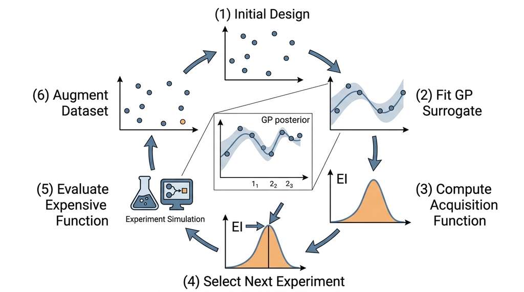
With a toolkit of acquisition functions in hand, each encoding a different stance on exploration versus exploitation, the remaining step is to wire the surrogate and the acquisition function into a closed loop that iterates automatically. Figure 5.5 illustrates this loop.

6. The Active Learning Loop

Putting everything together, the active learning loop for surrogate-based discovery has the following structure:

1. Initialize: Evaluate the expensive function at a small space-filling design \(\mathcal{D}_0 = \{(\mathbf{x}_i, y_i)\}_{i=1}^{N_0}\).
2. Fit surrogate: Train a GP on \(\mathcal{D}_t\) (the current dataset at iteration \(t\)).
3. Select next experiment: Maximize the acquisition function \(\alpha(\mathbf{x})\) over the input domain to find \(\mathbf{x}_{t+1}^* = \arg\max_{\mathbf{x}} \alpha(\mathbf{x})\).
4. Evaluate: Run the expensive function (simulator or physical experiment) at \(\mathbf{x}_{t+1}^*\) to obtain \(y_{t+1} = f(\mathbf{x}_{t+1}^*)\).
5. Augment: Add \((\mathbf{x}_{t+1}^*, y_{t+1})\) to \(\mathcal{D}_{t+1}\).
6. Check stopping criterion: If the budget is exhausted or the acquisition function's maximum drops below a threshold, stop. Otherwise, go to step 2.

This loop is the algorithmic skeleton of Bayesian optimization and the core of the Discovery Workbench's experiment selection module. Figure 5.3.1 illustrates active learning loop with GP surrogate and acquisition function.