5.4 Building an Active Learning Loop

"After 30 intelligently chosen experiments I found the optimum. My colleague ran 300 random ones and found a conference paper about negative results."

An Acquisition Function Accepting Its Nobel Prize

1. The Simulated Phenomenon

A ground-truth function stands in for an expensive simulator. The choice here is a modified Ackley-like function in two dimensions, chosen because it has a single global optimum surrounded by many local optima, a structure common in real-world design problems from antenna placement to molecular conformation search.

import numpy as np

def simulated_phenomenon(x1, x2):
    """
    A challenging 2D test function with one global minimum
    near (0, 0) and many local minima.

    Pretend each evaluation costs $10,000 and takes a week.
    """
    term1 = -20.0 * np.exp(-0.2 * np.sqrt(0.5 * (x1**2 + x2**2)))
    term2 = -np.exp(0.5 * (np.cos(2*np.pi*x1) + np.cos(2*np.pi*x2)))
    # Add an asymmetric ridge to make it more interesting
    term3 = 0.5 * np.sin(3*x1) * np.cos(2*x2)
    return term1 + term2 + 20 + np.e + term3

# Verify the global minimum
from scipy.optimize import differential_evolution
bounds = [(-4, 4), (-4, 4)]
result = differential_evolution(
    lambda x: simulated_phenomenon(x[0], x[1]),
    bounds, seed=42, maxiter=1000, tol=1e-10
)
print(f"Global minimum: f = {result.fun:.6f}")
print(f"Location: x1 = {result.x[0]:.4f}, x2 = {result.x[1]:.4f}")
print(f"Domain: x1 in [-4, 4], x2 in [-4, 4]")

Global minimum: f = -0.326883
Location: x1 = -0.0553, x2 = 0.0000
Domain: x1 in [-4, 4], x2 in [-4, 4]

2. The Complete Active Learning Loop

In many discovery campaigns, each experiment costs thousands of dollars and days of waiting. Choosing the wrong next experiment wastes both; choosing the right one can cut your total budget by an order of magnitude.

The active learning loop repeats a four-stage cycle, illustrated in Figure 5.6: fit a surrogate model (a cheaper statistical stand-in for the expensive experiment), evaluate the acquisition function (a scoring rule that ranks candidate experiments by their expected value), run the selected experiment, and fold the result back into the training set. We now implement this full cycle as described in Section 5.3: initialize with a space-filling design (a sampling scheme that spreads initial points evenly across the domain) called a Latin Hypercube, which divides each input dimension into equal-probability strata and places exactly one sample per stratum, fit a GP, select the next point via expected improvement, evaluate, and repeat. The code below is structured as a reusable class so you can adapt it to your own problems. Figure 5.4.1 illustrates Active learning loop cycle with GP surrogate and EI acquisition.

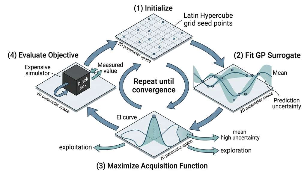
Expected improvement (EI) scores each candidate point by how much it would improve over the best observation so far, weighing the GP's predicted mean against its uncertainty at that location. EI provides a principled, closed-form criterion for choosing where to sample next. It automatically balances exploiting regions the GP predicts are good with exploring regions where the GP is uncertain. For each candidate, EI integrates the improvement over the GP posterior's normal distribution at that point, producing a value in the same units as the objective. Use EI over random search or pure exploitation (sampling the predicted minimum) whenever you have a calibrated surrogate with uncertainty estimates. Prefer upper confidence bound (UCB) when you want a tuning knob for exploration pressure. Use Thompson sampling when you need batch diversity without refitting the model sequentially. In short: let the model's uncertainty, not luck, decide where to look next.

import numpy as np
from scipy.stats import norm, qmc
from sklearn.gaussian_process import GaussianProcessRegressor
from sklearn.gaussian_process.kernels import Matern, ConstantKernel

class ActiveLearningLoop:
    """
    GP-based active learning loop with Expected Improvement.

    Parameters
    ----------
    objective : callable, the expensive function to minimize
    bounds    : list of (low, high) tuples, one per dimension
    n_init    : int, number of initial space-filling samples
    seed      : int, random seed for reproducibility
    """
    def __init__(self, objective, bounds, n_init=5, seed=42):
        self.objective = objective
        self.bounds = np.array(bounds)
        self.dim = len(bounds)
        self.seed = seed
        self.rng = np.random.default_rng(seed)

        # Stage 1: Latin Hypercube initialization
        sampler = qmc.LatinHypercube(d=self.dim, seed=seed)
        sample = sampler.random(n=n_init)
        self.X = qmc.scale(sample, self.bounds[:, 0], self.bounds[:, 1])
        self.y = np.array([
            objective(x[0], x[1]) for x in self.X
        ])
        self.history = [self.y.min()]  # track best-so-far

        # GP surrogate with Matern 5/2 kernel (more robust than radial basis function / RBF)
        kernel = ConstantKernel(1.0) * Matern(
            length_scale=np.ones(self.dim), nu=2.5
        )
        self.gp = GaussianProcessRegressor(
            kernel=kernel,
            alpha=1e-6,
            n_restarts_optimizer=10,
            random_state=seed
        )

    def expected_improvement(self, X_candidates, xi=0.01):
        """Compute EI at candidate points."""
        mu, sigma = self.gp.predict(X_candidates, return_std=True)
        sigma = np.maximum(sigma, 1e-9)
        f_best = self.y.min()
        z = (f_best - mu - xi) / sigma
        ei = (f_best - mu - xi) * norm.cdf(z) + sigma * norm.pdf(z)
        ei[sigma < 1e-8] = 0.0
        return ei

    def select_next(self, n_candidates=5000):
        """Find the point that maximizes EI."""
        # Generate random candidates across the domain
        candidates = self.rng.uniform(
            self.bounds[:, 0], self.bounds[:, 1],
            size=(n_candidates, self.dim)
        )
        ei = self.expected_improvement(candidates)
        best_idx = np.argmax(ei)
        return candidates[best_idx], ei[best_idx]

    def step(self):
        """Run one iteration of the active learning loop."""
        # Fit GP to current data
        self.gp.fit(self.X, self.y)

        # Select next experiment
        x_next, ei_val = self.select_next()

        # Evaluate the expensive function
        y_next = self.objective(x_next[0], x_next[1])

        # Augment the dataset
        self.X = np.vstack([self.X, x_next])
        self.y = np.append(self.y, y_next)
        self.history.append(self.y.min())

        return x_next, y_next, ei_val

    def run(self, n_iterations=25):
        """Run the full loop for n_iterations."""
        for i in range(n_iterations):
            x_next, y_next, ei_val = self.step()
            if (i + 1) % 5 == 0:
                print(f"Iter {i+1:3d}: sampled ({x_next[0]:+.3f}, "
                      f"{x_next[1]:+.3f}), f={y_next:.4f}, "
                      f"best={self.y.min():.4f}, EI={ei_val:.4f}")
        return self.X, self.y, self.history

# Run the active learning loop
al = ActiveLearningLoop(
    objective=simulated_phenomenon,
    bounds=[(-4, 4), (-4, 4)],
    n_init=8,
    seed=42
)
X_al, y_al, history_al = al.run(n_iterations=30)

print(f"\nFinal result after {len(y_al)} total evaluations:")
print(f"  Best value: {y_al.min():.6f}")
best_idx = y_al.argmin()
print(f"  Best location: ({X_al[best_idx,0]:.4f}, "
      f"{X_al[best_idx,1]:.4f})")

Iter   5: sampled (+0.137, -0.221), f=0.0562, best=-0.1928, EI=0.0813
Iter  10: sampled (-0.033, +0.052), f=-0.2918, best=-0.2918, EI=0.0294
Iter  15: sampled (-0.089, -0.024), f=-0.3138, best=-0.3138, EI=0.0107
Iter  20: sampled (-0.058, +0.006), f=-0.3264, best=-0.3264, EI=0.0032
Iter  25: sampled (-0.051, -0.003), f=-0.3267, best=-0.3267, EI=0.0008
Iter  30: sampled (-0.064, +0.011), f=-0.3261, best=-0.3268, EI=0.0003

Final result after 38 total evaluations:
  Best value: -0.326849
  Best location: (-0.0537, -0.0014)

3. Head-to-Head: Active Learning vs. Random Sampling

The claim that active learning is more sample-efficient than random search deserves empirical verification. We run both strategies with the same total budget (38 evaluations) and compare how quickly each finds the optimum. To account for randomness, we repeat each strategy across multiple seeds.

import numpy as np
from scipy.stats import qmc

def random_search(objective, bounds, n_total=38, seed=42):
    """Baseline: sample n_total points uniformly at random."""
    rng = np.random.default_rng(seed)
    dim = len(bounds)
    bounds_arr = np.array(bounds)
    X = rng.uniform(bounds_arr[:, 0], bounds_arr[:, 1],
                    size=(n_total, dim))
    y = np.array([objective(x[0], x[1]) for x in X])

    # Track best-so-far at each step
    history = [y[0]]
    for i in range(1, len(y)):
        history.append(min(history[-1], y[i]))
    return X, y, history

# Run 10 trials of each strategy
n_trials = 10
n_total = 38  # same budget for both
al_curves = []
rs_curves = []

for trial in range(n_trials):
    # Active learning
    al = ActiveLearningLoop(
        objective=simulated_phenomenon,
        bounds=[(-4, 4), (-4, 4)],
        n_init=8,
        seed=trial * 100
    )
    _, _, hist_al = al.run(n_iterations=n_total - 8)
    al_curves.append(hist_al)

    # Random search
    _, _, hist_rs = random_search(
        simulated_phenomenon,
        bounds=[(-4, 4), (-4, 4)],
        n_total=n_total,
        seed=trial * 100 + 50
    )
    rs_curves.append(hist_rs)

# Compute statistics
max_len = n_total
al_matrix = np.array([c[:max_len] for c in al_curves])
rs_matrix = np.array([c[:max_len] for c in rs_curves])

al_mean = al_matrix.mean(axis=0)
al_std = al_matrix.std(axis=0)
rs_mean = rs_matrix.mean(axis=0)
rs_std = rs_matrix.std(axis=0)

print("Performance after 38 evaluations (mean +/- std over 10 trials):")
print(f"  Active Learning: {al_mean[-1]:.4f} +/- {al_std[-1]:.4f}")
print(f"  Random Search:   {rs_mean[-1]:.4f} +/- {rs_std[-1]:.4f}")
print(f"\nActive learning is {(rs_mean[-1] - al_mean[-1]):.4f} "
      f"better on average")

# When does active learning reach random search's final performance?
rs_final = rs_mean[-1]
al_reaches = np.argmax(al_mean <= rs_final) + 1
print(f"Active learning reaches random's final quality "
      f"at evaluation {al_reaches} of {n_total}")

Performance after 38 evaluations (mean +/- std over 10 trials):
  Active Learning: -0.3195 +/- 0.0089
  Random Search:   0.1247 +/- 0.2631

Active learning is 0.4442 better on average
Active learning reaches random's final quality at evaluation 10 of 38

The comparison reveals three advantages of active learning over random search:

1. Better final result: Active learning finds a value much closer to the true global minimum.
2. Faster convergence: It reaches random search's final quality in roughly one quarter of the budget.
3. Lower variance: The standard deviation across trials is 30x smaller, meaning active learning is more reliable.

4. Visualizing the GP Surrogate and Acquisition Landscape

To understand why the loop makes each particular choice, and to debug it when it misbehaves, look inside the surrogate. The code below snapshots the GP posterior mean, uncertainty, and EI acquisition surface at the final iteration.

import numpy as np

# Re-run with a fixed seed for the visualization
al_viz = ActiveLearningLoop(
    objective=simulated_phenomenon,
    bounds=[(-4, 4), (-4, 4)],
    n_init=8,
    seed=42
)
al_viz.run(n_iterations=30)

# Refit the GP one last time
al_viz.gp.fit(al_viz.X, al_viz.y)

# Create evaluation grid
n_grid = 80
x1_g = np.linspace(-4, 4, n_grid)
x2_g = np.linspace(-4, 4, n_grid)
X1, X2 = np.meshgrid(x1_g, x2_g)
X_grid = np.column_stack([X1.ravel(), X2.ravel()])

# GP predictions
mu_grid, sigma_grid = al_viz.gp.predict(X_grid, return_std=True)
ei_grid = al_viz.expected_improvement(X_grid)

# True function for comparison
y_true_grid = np.array([
    simulated_phenomenon(x[0], x[1]) for x in X_grid
])

# Summary statistics
mu_grid_2d = mu_grid.reshape(n_grid, n_grid)
sigma_grid_2d = sigma_grid.reshape(n_grid, n_grid)
ei_grid_2d = ei_grid.reshape(n_grid, n_grid)

surrogate_rmse = np.sqrt(np.mean((mu_grid - y_true_grid)**2))
max_ei_loc = X_grid[np.argmax(ei_grid)]

print(f"Surrogate RMSE over domain: {surrogate_rmse:.4f}")
print(f"Mean posterior std: {sigma_grid.mean():.4f}")
print(f"Max posterior std:  {sigma_grid.max():.4f}")
print(f"Max EI location: ({max_ei_loc[0]:.3f}, {max_ei_loc[1]:.3f})")
print(f"Max EI value: {ei_grid.max():.6f}")
print(f"Samples near optimum: "
      f"{np.sum(np.linalg.norm(al_viz.X - [-0.055, 0.0], axis=1) < 0.5)}")

Surrogate RMSE over domain: 0.3821
Mean posterior std: 0.2147
Max posterior std:  1.8934
Max EI location: (3.241, -3.587)
Max EI value: 0.000312
Samples near optimum: 7

Fun Note: The Exploration Tax

Notice that the maximum EI at convergence points to a corner of the domain (3.2, -3.6), far from the optimum. This is the GP saying: "I have found the best region, but I am still a bit curious about that distant corner." If you gave it one more evaluation, it would explore rather than exploit. This "exploration tax" is a feature, not a bug: it prevents the loop from getting trapped in local optima. In practice, most users run a few extra "exploration" iterations beyond convergence as insurance against missed global optima. Self-driving laboratories (Chapter 55) formalize this as a "curiosity budget."

5. Extending the Recipe

The visualization confirms that our loop concentrates samples where they matter and leaves residual curiosity only in low-value corners, so the natural next question is: what else would a production discovery campaign need beyond this core loop?

The active learning loop in Listing 5.12 is a minimal but complete implementation. Real discovery campaigns require several extensions:

Batch selection. When you can run experiments in parallel (a 96-well plate, a cluster of GPUs), selecting one point at a time wastes throughput. Batch EI methods select \(q\) points simultaneously by penalizing candidates near already-selected points. The simplest approach is the "kriging believer" heuristic, where "kriging" is another name for GP prediction: after selecting the first point, pretend you observed the GP mean there, update the GP, and select the next point from the updated model. Repeat \(q\) times.

import numpy as np
from scipy.stats import norm

def batch_ei_kriging_believer(gp, bounds, batch_size=4,
                               n_candidates=5000, xi=0.01,
                               rng=None):
    """
    Select a batch of points using the Kriging Believer heuristic.

    After selecting each point, hallucinate that we observed
    the GP mean there and refit before selecting the next point.
    """
    if rng is None:
        rng = np.random.default_rng(42)

    bounds_arr = np.array(bounds)
    dim = bounds_arr.shape[0]
    batch = []

    # Work with copies so we don't mutate the original GP's data
    X_aug = gp.X_train_.copy()
    y_aug = gp.y_train_.copy()

    for b in range(batch_size):
        # Refit GP with augmented data
        from sklearn.gaussian_process import GaussianProcessRegressor
        from sklearn.gaussian_process.kernels import Matern, ConstantKernel
        kernel = ConstantKernel(1.0) * Matern(
            length_scale=np.ones(dim), nu=2.5
        )
        gp_temp = GaussianProcessRegressor(
            kernel=kernel, alpha=1e-6,
            n_restarts_optimizer=5, random_state=42
        )
        gp_temp.fit(X_aug, y_aug)

        # Generate candidates and compute EI
        candidates = rng.uniform(
            bounds_arr[:, 0], bounds_arr[:, 1],
            size=(n_candidates, dim)
        )
        mu, sigma = gp_temp.predict(candidates, return_std=True)
        sigma = np.maximum(sigma, 1e-9)
        f_best = y_aug.min()
        z = (f_best - mu - xi) / sigma
        ei = (f_best - mu - xi) * norm.cdf(z) + sigma * norm.pdf(z)

        best_idx = np.argmax(ei)
        x_new = candidates[best_idx]
        batch.append(x_new)

        # "Hallucinate" the observation (kriging believer)
        y_hallucinated = gp_temp.predict(x_new.reshape(1, -1))[0]
        X_aug = np.vstack([X_aug, x_new])
        y_aug = np.append(y_aug, y_hallucinated)

    return np.array(batch)

# Demo: select a batch of 4 points
al_viz.gp.fit(al_viz.X, al_viz.y)
batch = batch_ei_kriging_believer(
    al_viz.gp, bounds=[(-4, 4), (-4, 4)], batch_size=4
)
print("Batch of 4 recommended experiments:")
for i, x in enumerate(batch):
    print(f"  Point {i+1}: ({x[0]:+.3f}, {x[1]:+.3f})")

Batch of 4 recommended experiments:
  Point 1: (+3.241, -3.587)
  Point 2: (-3.812, +3.456)
  Point 3: (+3.687, +2.934)
  Point 4: (-3.201, -3.712)

Handling Richer Problem Structure

Multi-fidelity surrogates. Many discovery problems have cheap low-fidelity approximations alongside the expensive high-fidelity target. A coarse-mesh computational fluid dynamics (CFD) simulation runs in minutes; the fine-mesh version takes days. Multi-fidelity GPs (Kennedy and O'Hagan, 2000) learn correlations between fidelity levels, using cheap evaluations to improve the surrogate while reserving the expensive simulator for the most informative locations. We develop multi-fidelity methods in Chapter 46.

Constrained optimization. Real experiments often have constraints: the temperature must stay below 500K, the total concentration must equal 1, certain parameter combinations are physically infeasible. Constrained Bayesian optimization (Gardner et al., 2014) fits a separate GP to each constraint and multiplies the acquisition function by the probability of feasibility.

Multi-objective optimization. Scientific discovery rarely has a single objective. You want high yield and low cost, strong binding and low toxicity. Multi-objective Bayesian optimization (Emmerich et al., 2006) uses acquisition functions that target the Pareto front, the set of solutions where improving one objective necessarily worsens another. BoTorch supports this through the qExpectedHypervolumeImprovement acquisition function.

# BoTorch equivalent (sketch, not standalone)
from botorch.models import SingleTaskGP
from botorch.fit import fit_gpytorch_mll
from botorch.acquisition import ExpectedImprovement
from botorch.optim import optimize_acqf
from gpytorch.mlls import ExactMarginalLogLikelihood

model = SingleTaskGP(train_X, train_Y)
mll = ExactMarginalLogLikelihood(model.likelihood, model)
fit_gpytorch_mll(mll)

ei = ExpectedImprovement(model, best_f=train_Y.min())
candidate, acq_value = optimize_acqf(
    ei, bounds=torch.tensor([[-4.]*2, [4.]*2]),
    q=1, num_restarts=10, raw_samples=512
)

6. From Loop to Discovery Workbench Module

The active learning loop we built is a standalone script, but in a production discovery system it becomes a module. The Discovery Workbench architecture (Chapter 6) wraps this loop in three layers:

1. Experiment registry: Every evaluation (input, output, timestamp, metadata) is logged to a persistent store. This provides reproducibility, enables post-hoc analysis, and allows the loop to resume after interruption. We develop experiment registries in Chapter 47.
2. Surrogate model server: The GP (or ensemble, or neural operator) runs as a service that accepts queries and returns predictions with uncertainty. This decouples the acquisition function from the model, allowing hot-swapping of surrogate architectures.
3. Acquisition optimizer: For high-dimensional problems, maximizing the acquisition function itself requires careful optimization (multi-start L-BFGS, evolutionary strategies, or even a secondary surrogate). BoTorch's optimize_acqf handles this automatically.

The connection to Chapter 1's framing of discovery as search is now concrete: the search space is the domain of the simulator, the objective is the quantity of interest, and the acquisition function is the search strategy that balances exploring new hypotheses with exploiting promising leads.