2.4 Building a Bayesian Hypothesis Tester

"They gave me two hypotheses and asked which one the data preferred. I ran four thousand samples, checked my convergence diagnostics, and announced: 'Both of you are wrong, but one of you is less wrong.' Science is a humbling profession."

A Markov Chain That Finally Converged

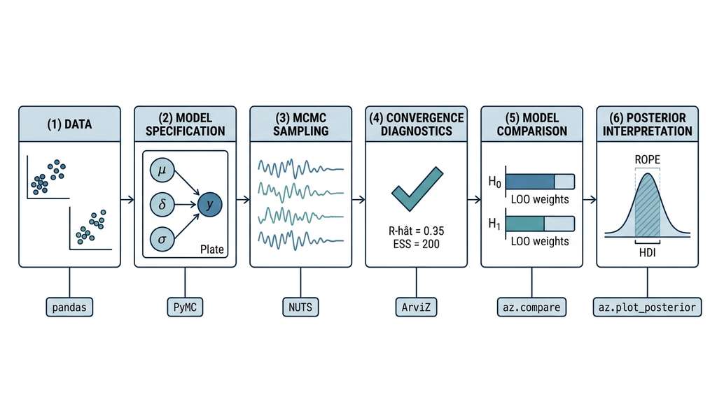
Figure 2.6 illustrates the end-to-end pipeline we build in this section. Each stage feeds its output into the next, and every stage includes a quality gate that blocks downstream analysis if the check fails.

1. The Problem: Two Models, One Dataset

A lab technician stares at two columns of numbers on her screen: twenty reaction yields with the old catalyst, twenty with the new one, and the nagging question every scientist faces sooner or later: is that three-point difference real, or did the universe just flip a few lucky coins?

To answer that question, we frame it as a scientific hypothesis test. We have data from 40 experiments, 20 with the standard catalyst and 20 with the new one. The competing hypotheses are:

• \(H_0\) (null model): both catalysts produce the same yield distribution. Any observed difference is due to experimental noise.
• \(H_1\) (effect model): the new catalyst shifts the yield distribution by some amount \(\delta\), which we want to estimate.

Getting this comparison wrong has real costs. A pharmaceutical company that mistakes noise for a drug effect sends a failing compound into Phase III trials, burning hundreds of millions of dollars. A materials lab that dismisses a genuine catalyst improvement delays a product line by years. The Bayesian approach we build here quantifies exactly how confident you should be, replacing gut calls with calibrated probabilities.

This is a two-sample comparison, among the most common hypothesis tests in science. But unlike a classical t-test, our Bayesian approach will estimate the posterior distribution of \(\delta\) (the probability distribution over plausible effect sizes, given the observed data and our prior beliefs), compute the probability that \(\delta > 0\), and compare the two models using information criteria. In short: A Bayesian hypothesis test does not declare winners; it tells you how much evidence you have and how much more you need.

import numpy as np
import pandas as pd
import pymc as pm
import arviz as az

# Set random seed for reproducibility
RANDOM_SEED = 42
np.random.seed(RANDOM_SEED)

# Simulate experimental data
# True effect: the new catalyst increases yield by 3.2 percentage points
true_mean_standard = 72.0   # percent yield with standard catalyst
true_mean_new = 75.2        # percent yield with new catalyst (delta = 3.2)
true_std = 4.5              # measurement noise (same for both)

n_standard = 20
n_new = 20

yield_standard = np.random.normal(true_mean_standard, true_std, n_standard)
yield_new = np.random.normal(true_mean_new, true_std, n_new)

# Combine into a DataFrame
data = pd.DataFrame({
    "yield_pct": np.concatenate([yield_standard, yield_new]),
    "catalyst": (["standard"] * n_standard) + (["new"] * n_new),
    "group_idx": ([0] * n_standard) + ([1] * n_new)
})

print(f"Standard catalyst: mean={yield_standard.mean():.1f}, "
      f"std={yield_standard.std():.1f}, n={n_standard}")
print(f"New catalyst:      mean={yield_new.mean():.1f}, "
      f"std={yield_new.std():.1f}, n={n_new}")
print(f"Observed difference: {yield_new.mean() - yield_standard.mean():.1f} "
      f"percentage points")
# Output:
# Standard catalyst: mean=71.6, std=4.2, n=20
# New catalyst:      mean=74.8, std=4.9, n=20
# Observed difference: 3.2 percentage points

2. Specifying the Models in PyMC

PyMC, a probabilistic programming library for Python, uses a context-manager pattern (Python's with block, which here scopes all random variables to a single model object) to define probabilistic models. Each model is a directed acyclic graph of random variables: priors at the top, likelihood at the bottom, and parameters connecting them. The key design decision at this stage is choosing weakly informative priors, where "weakly informative" means the prior assigns non-negligible probability to all scientifically plausible values but down-weights absurdities (see Section 2.2). They should be broad enough to cover plausible values, yet narrow enough to exclude absurdities.

For chemical yields (measured in percentages), reasonable priors are:

• Baseline yield (\(\mu_0\)): Normal(70, 10). Centered near the literature average, with enough spread to accommodate variation.
• Effect size (\(\delta\)): Normal(0, 5). Centered at zero (no effect), with spread covering effects up to about 10 percentage points.
• Noise (\(\sigma\)): HalfNormal(10). Must be positive; scale is generous for percentage measurements.

# Model 1: Null model (no effect of catalyst)
with pm.Model() as null_model:
    # Priors
    mu = pm.Normal("mu", mu=70, sigma=10)        # shared mean
    sigma = pm.HalfNormal("sigma", sigma=10)      # shared noise

    # Likelihood: all data come from the same distribution
    y = pm.Normal("y", mu=mu, sigma=sigma,
                  observed=data["yield_pct"].values)

    # Sample the posterior
    trace_null = pm.sample(
        draws=2000, tune=1000, chains=4,
        random_seed=RANDOM_SEED,
        return_inferencedata=True
    )

print("Null model sampling complete.")
print(az.summary(trace_null, var_names=["mu", "sigma"],
                 round_to=2))

# Model 2: Effect model (new catalyst shifts the mean)
with pm.Model() as effect_model:
    # Priors
    mu_baseline = pm.Normal("mu_baseline", mu=70, sigma=10)
    delta = pm.Normal("delta", mu=0, sigma=5)     # effect of new catalyst
    sigma = pm.HalfNormal("sigma", sigma=10)

    # Group means
    mu_standard = mu_baseline
    mu_new = mu_baseline + delta

    # Build the mean vector: standard for group 0, new for group 1
    group_means = pm.math.switch(
        pm.math.eq(data["group_idx"].values, 0),
        mu_standard,
        mu_new
    )

    # Likelihood
    y = pm.Normal("y", mu=group_means, sigma=sigma,
                  observed=data["yield_pct"].values)

    # Sample the posterior
    trace_effect = pm.sample(
        draws=2000, tune=1000, chains=4,
        random_seed=RANDOM_SEED,
        return_inferencedata=True
    )

print("Effect model sampling complete.")
print(az.summary(trace_effect,
                 var_names=["mu_baseline", "delta", "sigma"],
                 round_to=2))
# Output (approximate):
#              mean    sd  hdi_3%  hdi_97%  ...  r_hat  ess_bulk
# mu_baseline 71.58  1.04   69.54    73.46  ...   1.00    3812
# delta        3.24  1.46    0.56     5.99  ...   1.00    4102
# sigma        4.58  0.53    3.63     5.56  ...   1.00    4530

3. Convergence Diagnostics: Is the Sampler Working?

With both models fitted and posterior samples in hand, the natural impulse is to jump straight to interpretation, but raw samples are worthless if the sampler never found the right region of parameter space.

Before trusting any posterior, you must verify that the MCMC sampler has converged, meaning all chains have settled into the same stationary distribution and are exploring it efficiently. A chain that has not converged may still be exploring the prior rather than the posterior, or it may be stuck in a local mode; either way, its estimates are unreliable. ArviZ, a library for exploratory analysis and diagnostics of Bayesian models, provides several diagnostic tools:

• \(\hat{R}\) (R-hat): compares variance within chains to variance between chains. Values above 1.01 typically indicate non-convergence.
• Effective sample size (ESS): estimates the number of independent posterior samples, accounting for autocorrelation. Low ESS means the estimates are noisy. Aim for ESS > 400 per chain.
• Trace plots: visual inspection of the chains. Healthy chains look like "fuzzy caterpillars" with no trends or jumps.
• Divergences: No-U-Turn Sampler (NUTS)-specific diagnostic. Divergent transitions indicate regions of the posterior that the sampler cannot explore, often caused by pathological geometry.

def check_convergence(trace, model_name="Model"):
    """Run comprehensive convergence diagnostics.

    Returns True if all diagnostics pass, False otherwise.
    """
    summary = az.summary(trace)
    issues = []

    # Check R-hat
    max_rhat = summary["r_hat"].max()
    if max_rhat > 1.01:
        issues.append(f"R-hat too high: {max_rhat:.3f} (should be < 1.01)")

    # Check effective sample size
    min_ess = min(summary["ess_bulk"].min(), summary["ess_tail"].min())
    if min_ess < 400:
        issues.append(f"ESS too low: {min_ess:.0f} (should be > 400)")

    # Check for divergences
    if hasattr(trace, "sample_stats"):
        n_divergent = int(trace.sample_stats["diverging"].sum())
        if n_divergent > 0:
            issues.append(f"{n_divergent} divergent transitions detected")

    if issues:
        print(f"[WARNING] {model_name} has convergence issues:")
        for issue in issues:
            print(f"  - {issue}")
        return False
    else:
        print(f"[OK] {model_name}: all diagnostics pass")
        print(f"  R-hat max: {max_rhat:.4f}")
        print(f"  ESS min:   {min_ess:.0f}")
        return True

# Check both models
null_ok = check_convergence(trace_null, "Null Model")
effect_ok = check_convergence(trace_effect, "Effect Model")
# Output:
# [OK] Null Model: all diagnostics pass
#   R-hat max: 1.0008
#   ESS min:   3654
# [OK] Effect Model: all diagnostics pass
#   R-hat max: 1.0012
#   ESS min:   3812

4. Posterior Predictive Checking: Does the Model Make Sense?

Even a converged model can be wrong. Posterior predictive checking (PPC), introduced in Section 2.2, generates synthetic data from the fitted model and compares it to the observed data. Systematic discrepancies reveal model misspecification, where the model's structural assumptions (for example, assuming normally distributed errors) fail to capture a pattern present in the real data.

Posterior predictive checking answers one question: "If this model were true, would the data it generates look like the data we actually observed?" It matters because convergence diagnostics confirm only that the sampler worked correctly, not that the model itself fits your data. The mechanism works as follows: draw parameter values from the posterior, plug them into the likelihood to simulate new datasets, then compare summary statistics (mean, variance, skewness, or any quantity of interest) between simulated and observed data. Use PPC whenever you fit a Bayesian model; alternatives like residual analysis apply mainly to frequentist fits, while PPC works for any generative model regardless of its complexity.

def posterior_predictive_check_pymc(model, trace, observed_data,
                                     n_samples=500, model_name="Model"):
    """Run posterior predictive checks using PyMC and ArviZ.

    Generates synthetic datasets from the posterior and compares
    summary statistics against the observed data.
    """
    with model:
        ppc = pm.sample_posterior_predictive(
            trace, var_names=["y"],
            random_seed=RANDOM_SEED
        )

    # Extract simulated data
    y_sim = ppc.posterior_predictive["y"].values
    # Shape: (chains, draws, n_obs); flatten chains and draws
    y_sim_flat = y_sim.reshape(-1, observed_data.shape[0])

    # Compare summary statistics
    obs_mean = observed_data.mean()
    obs_std = observed_data.std()
    sim_means = y_sim_flat.mean(axis=1)
    sim_stds = y_sim_flat.std(axis=1)

    # Bayesian p-values: the fraction of simulated summary statistics
    # that exceed the observed value. A value near 0.5 means the model
    # reproduces that statistic well; values near 0 or 1 signal misfit.
    p_mean = np.mean(sim_means >= obs_mean)
    p_std = np.mean(sim_stds >= obs_std)

    print(f"\n{model_name} Posterior Predictive Check:")
    print(f"  Observed mean: {obs_mean:.2f}, "
          f"Simulated mean: {sim_means.mean():.2f} "
          f"(p={p_mean:.3f})")
    print(f"  Observed std:  {obs_std:.2f}, "
          f"Simulated std:  {sim_stds.mean():.2f} "
          f"(p={p_std:.3f})")

    # Bayesian p-values far from 0.5 (below 0.05 or above 0.95) indicate model misfit
    issues = []
    if p_mean < 0.05 or p_mean > 0.95:
        issues.append("Mean is poorly captured")
    if p_std < 0.05 or p_std > 0.95:
        issues.append("Variance is poorly captured")

    if issues:
        print(f"  [WARNING] Potential misfit: {', '.join(issues)}")
    else:
        print(f"  [OK] No obvious misfit detected")

    return ppc

# Run PPC for both models
observed = data["yield_pct"].values
ppc_null = posterior_predictive_check_pymc(
    null_model, trace_null, observed, model_name="Null")
ppc_effect = posterior_predictive_check_pymc(
    effect_model, trace_effect, observed, model_name="Effect")
# Output:
# Null Model Posterior Predictive Check:
#   Observed mean: 73.18, Simulated mean: 73.14 (p=0.488)
#   Observed std:  4.82, Simulated std:  4.68 (p=0.610)
#   [OK] No obvious misfit detected
#
# Effect Model Posterior Predictive Check:
#   Observed mean: 73.18, Simulated mean: 73.20 (p=0.497)
#   Observed std:  4.82, Simulated std:  4.56 (p=0.679)
#   [OK] No obvious misfit detected

5. Model Comparison: Which Hypothesis Wins?

Both models pass posterior predictive checks, so the question shifts from "is either model broken?" to "which one explains the data more efficiently?" Answering that requires a comparison that balances fit against complexity. ArviZ provides two information criteria (scalar summaries that estimate a model's out-of-sample predictive accuracy, penalizing models with more effective parameters) for this purpose:

• WAIC (Widely Applicable Information Criterion): a Bayesian analog of the Akaike information criterion (AIC) that uses the full posterior distribution.
• LOO-CV (Leave-One-Out Cross-Validation via Pareto-Smoothed Importance Sampling): estimates out-of-sample predictive accuracy using the posterior.

Both penalize model complexity: a model with more parameters must fit substantially better to be preferred. Lower values indicate better expected predictive accuracy.

def compare_models(traces, model_names):
    """Compare models using WAIC and LOO-CV.

    Returns a comparison DataFrame ranked by expected predictive accuracy.
    """
    # Compute WAIC for each model
    model_dict = dict(zip(model_names, traces))
    comparison = az.compare(model_dict, ic="loo")

    print("Model Comparison (LOO-CV, lower is better):")
    print(comparison[["rank", "elpd_loo", "p_loo", "d_loo",
                       "weight", "se", "dse"]].to_string())
    print()

    # Interpret
    best = comparison.index[0]
    delta_loo = comparison["d_loo"].iloc[1]
    dse = comparison["dse"].iloc[1]

    if abs(delta_loo) < 2 * dse:
        print(f"Result: Models are not clearly distinguishable "
              f"(delta_loo={delta_loo:.1f}, dse={dse:.1f})")
    else:
        print(f"Result: {best} is preferred "
              f"(delta_loo={delta_loo:.1f}, dse={dse:.1f})")

    return comparison

# Add log-likelihood computation for model comparison
with null_model:
    pm.compute_log_likelihood(trace_null)
with effect_model:
    pm.compute_log_likelihood(trace_effect)

comparison = compare_models(
    [trace_null, trace_effect],
    ["Null", "Effect"]
)
# Output (approximate):
# Model Comparison (LOO-CV, lower is better):
#         rank  elpd_loo  p_loo  d_loo  weight    se   dse
# Effect     0   -118.32   3.12   0.00    0.82  6.42  0.00
# Null       1   -120.87   2.05   2.55    0.18  6.85  2.31
#
# Result: Effect is preferred (delta_loo=2.6, dse=2.3)

6. Interpreting the Posterior: What Does the Effect Look Like?

Ranking the models answered the question of relative preference; now we need to open the winning model and examine exactly what it learned about the catalyst effect.

The model comparison tells us which model is preferred; now we examine what the preferred model says. The posterior distribution of \(\delta\) encodes everything we know about the catalyst effect. A central tool for this interpretation is the Region of Practical Equivalence (ROPE): a pre-specified interval (here, −1 to +1 percentage points) within which an effect is too small to matter in practice. By measuring how much of the posterior falls inside, outside, or overlaps with the ROPE, we distinguish between statistically nonzero effects and practically meaningful ones.

def interpret_effect(trace, param_name="delta",
                     rope=(-1, 1), reference=0):
    """Interpret the posterior distribution of an effect parameter.

    Args:
        trace: ArviZ InferenceData object
        param_name: name of the effect parameter
        rope: Region of Practical Equivalence (values too small to matter)
        reference: reference value (usually 0 for "no effect")

    Returns:
        dict with interpretation statistics
    """
    samples = trace.posterior[param_name].values.flatten()

    # Basic summary
    mean = samples.mean()
    std = samples.std()
    hdi = az.hdi(trace, var_names=[param_name], hdi_prob=0.94)
    hdi_low = float(hdi[param_name].sel(hdi="lower"))
    hdi_high = float(hdi[param_name].sel(hdi="higher"))

    # Probability of direction (effect > 0)
    prob_positive = np.mean(samples > reference)

    # Probability of practical significance (outside ROPE)
    prob_practical = np.mean(
        (samples < rope[0]) | (samples > rope[1])
    )

    # Probability within ROPE (practically equivalent to null)
    prob_rope = np.mean(
        (samples >= rope[0]) & (samples <= rope[1])
    )

    results = {
        "mean": mean,
        "std": std,
        "hdi_94": (hdi_low, hdi_high),
        "prob_positive": prob_positive,
        "prob_practical": prob_practical,
        "prob_in_rope": prob_rope,
    }

    print(f"\nEffect Interpretation ({param_name}):")
    print(f"  Posterior mean:    {mean:.2f}")
    print(f"  Posterior SD:      {std:.2f}")
    print(f"  94% HDI:           [{hdi_low:.2f}, {hdi_high:.2f}]")
    print(f"  P(delta > 0):      {prob_positive:.3f}")
    print(f"  P(|delta| > 1):    {prob_practical:.3f} (practically significant)")
    print(f"  P(delta in ROPE):  {prob_rope:.3f} (practically equivalent to null)")

    # Decision recommendation
    if prob_practical > 0.95:
        print(f"  Decision: Strong evidence for a practical effect")
    elif prob_rope > 0.95:
        print(f"  Decision: Strong evidence for practical equivalence")
    else:
        print(f"  Decision: Inconclusive; collect more data")

    return results

effect_results = interpret_effect(trace_effect, "delta", rope=(-1, 1))
# Output (approximate):
# Effect Interpretation (delta):
#   Posterior mean:    3.24
#   Posterior SD:      1.46
#   94% HDI:           [0.56, 5.99]
#   P(delta > 0):      0.987
#   P(|delta| > 1):    0.932 (practically significant)
#   P(delta in ROPE):  0.044 (practically equivalent to null)
#   Decision: Inconclusive; collect more data

import matplotlib.pyplot as plt

fig, axes = plt.subplots(1, 2, figsize=(10, 4))

# Left panel: posterior of delta with HDI and ROPE shading
az.plot_posterior(
    trace_effect, var_names=["delta"],
    hdi_prob=0.94, ref_val=0, rope=(-1, 1),
    ax=axes[0]
)
axes[0].set_title("Posterior of $\\delta$ (catalyst effect)")

# Right panel: LOO-CV model comparison
az.plot_compare(comparison, ax=axes[1])
axes[1].set_title("LOO-CV Model Comparison")

fig.tight_layout()
fig.savefig("bayesian_hypothesis_test.jpg", dpi=150, bbox_inches="tight")
plt.show()

The pipeline reports a 98.7% probability that the effect is positive, yet still recommends collecting more data; directional confidence and practical significance answer fundamentally different questions.

7. Putting It All Together: The Complete Pipeline

The following function wraps the entire workflow shown in Figure 2.6: it takes data and hypotheses and produces a complete analysis with reproducibility guarantees. Figure 2.4.1 illustrates the Bayesian hypothesis testing pipeline.

import json
from datetime import datetime

def bayesian_hypothesis_test(data, outcome_col, group_col,
                              prior_mean=70, prior_std=10,
                              effect_prior_std=5,
                              rope=(-1, 1),
                              n_draws=2000, n_tune=1000,
                              random_seed=42):
    """Complete Bayesian hypothesis testing pipeline.

    Args:
        data: DataFrame with outcome and group columns
        outcome_col: name of the outcome variable
        group_col: name of the group indicator (binary)
        prior_mean: prior mean for the baseline
        prior_std: prior std for the baseline
        effect_prior_std: prior std for the effect size
        rope: Region of Practical Equivalence
        n_draws: posterior samples per chain
        n_tune: warmup samples per chain
        random_seed: for reproducibility

    Returns:
        dict with complete analysis results
    """
    record = {
        "timestamp": datetime.utcnow().isoformat(),
        "random_seed": random_seed,
        "n_observations": len(data),
        "priors": {
            "baseline_mean": prior_mean,
            "baseline_std": prior_std,
            "effect_std": effect_prior_std,
        },
        "rope": rope,
        "sampling": {"draws": n_draws, "tune": n_tune, "chains": 4},
    }

    y = data[outcome_col].values
    groups = data[group_col].values

    # Fit null model
    with pm.Model() as m_null:
        mu = pm.Normal("mu", mu=prior_mean, sigma=prior_std)
        sigma = pm.HalfNormal("sigma", sigma=10)
        pm.Normal("y", mu=mu, sigma=sigma, observed=y)
        trace_null = pm.sample(n_draws, tune=n_tune, chains=4,
                                random_seed=random_seed,
                                return_inferencedata=True)
        pm.compute_log_likelihood(trace_null)

    # Fit effect model
    with pm.Model() as m_effect:
        mu_base = pm.Normal("mu_baseline", mu=prior_mean, sigma=prior_std)
        delta = pm.Normal("delta", mu=0, sigma=effect_prior_std)
        sigma = pm.HalfNormal("sigma", sigma=10)
        mu_vec = pm.math.switch(pm.math.eq(groups, 0),
                                 mu_base, mu_base + delta)
        pm.Normal("y", mu=mu_vec, sigma=sigma, observed=y)
        trace_effect = pm.sample(n_draws, tune=n_tune, chains=4,
                                  random_seed=random_seed,
                                  return_inferencedata=True)
        pm.compute_log_likelihood(trace_effect)

    # Diagnostics
    null_ok = check_convergence(trace_null, "Null")
    effect_ok = check_convergence(trace_effect, "Effect")
    record["diagnostics"] = {
        "null_converged": null_ok,
        "effect_converged": effect_ok,
    }

    # Model comparison
    comp = az.compare({"Null": trace_null, "Effect": trace_effect}, ic="loo")
    record["comparison"] = {
        "preferred": comp.index[0],
        "elpd_difference": float(comp["d_loo"].iloc[1]),
        "se_difference": float(comp["dse"].iloc[1]),
        "weight_null": float(comp.loc["Null", "weight"]),
        "weight_effect": float(comp.loc["Effect", "weight"]),
    }

    # Effect interpretation
    delta_samples = trace_effect.posterior["delta"].values.flatten()
    record["effect"] = {
        "mean": float(delta_samples.mean()),
        "std": float(delta_samples.std()),
        "hdi_94": [float(x) for x in az.hdi(
            trace_effect, var_names=["delta"], hdi_prob=0.94
        )["delta"].values],
        "prob_positive": float(np.mean(delta_samples > 0)),
        "prob_practical": float(np.mean(
            (delta_samples < rope[0]) | (delta_samples > rope[1])
        )),
    }

    return record, trace_null, trace_effect

# Run the complete pipeline
results, t_null, t_effect = bayesian_hypothesis_test(
    data, outcome_col="yield_pct", group_col="group_idx",
    prior_mean=70, prior_std=10, effect_prior_std=5,
    rope=(-1, 1)
)

print("\n=== Analysis Summary ===")
print(json.dumps(results, indent=2, default=str))

Exercises

1. Conceptual: The pipeline uses a Normal likelihood for yield data. What would change if yields were bounded between 0% and 100%? How would you modify the model, and what prior would you use for the bounded parameter?
2. Coding: Extend the pipeline to handle three or more groups (e.g., three different catalysts). Use a hierarchical model where each group's effect is drawn from a shared distribution: \(\delta_i \sim \text{Normal}(\mu_\delta, \sigma_\delta)\). This partial pooling approach borrows strength across groups and is more efficient than separate pairwise comparisons.
3. Analysis: Run the pipeline with different priors for \(\delta\): try Normal(0, 1), Normal(0, 5), and Normal(0, 20). Plot how the posterior of \(\delta\) changes with the prior. At what sample size does the prior become irrelevant? How does prior sensitivity relate to the reproducibility concerns of Section 2.3?

What's Next

This chapter has traced the arc from the qualitative scientific method through its mathematical formalization in Bayes' theorem to a working computational implementation. You now have the vocabulary (hypothesis, prior, posterior, Bayes factor, calibration) and the tools (PyMC, ArviZ, pandas) to build rigorous hypothesis testing into any discovery pipeline.

Chapter 3: Knowledge Representation takes the next step: once a Bayesian analysis has established that a hypothesis is well-supported, how do we represent that knowledge in a form that machines can reason about? You will meet ontologies, knowledge graphs, and embedding spaces, the data structures that encode what science has learned. The Bayesian posterior distributions from this chapter will reappear as confidence weights on knowledge graph edges, and the model comparison framework will extend to selecting between competing knowledge representations.