"I am seven microservices in a trench coat pretending to be a scientist. The trench coat is YAML."
A Microservice That Achieved Consciousness
Prerequisites
This section assumes you have read Chapter 1 (discovery as search through hypothesis space), Chapter 3 (knowledge representation and ontologies), and Chapter 5 (the interplay of data, models, and simulation). You should be comfortable with Python dataclasses and type annotations. Familiarity with Pydantic and basic software architecture patterns (registries, dependency injection) will help, but we introduce each concept as it arises.
A discovery system is not a single program. It is a coordinated assembly of data stores, executable code, trained models, callable tools, autonomous agents, accumulated memory, and provenance records. Each of these responsibilities lives in its own layer, with typed interfaces connecting them. Getting the layer boundaries right determines whether your system can reproduce a result six months later, whether a new team member can trace a surprising finding back to its raw data, and whether an agent can safely extend the system without human supervision. This section maps the seven layers, defines their contracts, and shows what breaks when you skip one.
1. The Workbench as a Formal System
Three AI agents run parallel experiments overnight: one tests a drug combination, another re-analyzes last month's genomics data, and a third fine-tunes a model on freshly collected spectra. By morning each claims a breakthrough, but can you tell which results are trustworthy, which code produced them, and whether any agent silently reused corrupted data? A Discovery Workbench answers that question. It supports the full cycle introduced in Chapter 1 (formulating hypotheses, designing experiments, executing computations, analyzing results, and recording what happened) while keeping every piece traceable. We can formalize this as a seven-tuple:
A Discovery Workbench decomposes the scientific workflow into isolated, interchangeable layers. Each layer carries a typed contract, so you can swap, upgrade, or scale it independently. This matters because monolithic scripts that blend data loading, computation, and result storage become untraceable and unreproducible the moment a second person or a second machine joins the project. Each layer exposes a small set of abstract methods (register, retrieve, version, lineage) through Python protocols, where a protocol is a structural interface that defines a set of methods a class must implement without requiring explicit inheritance. Layers communicate only through these interfaces, never by sharing mutable state. You should reach for this layered design over a flat script whenever your work involves collaboration, automation, or any result you may need to reproduce later. For a quick one-off analysis you will never revisit, a single notebook remains perfectly adequate.
$$\mathcal{W} = (D, C, M, T, A, \Gamma, P)$$where \(D\) is the Data Layer (raw observations, curated datasets, and feature stores), \(C\) is the Code Layer (versioned scripts, notebooks, and pipelines), \(M\) is the Model Layer (trained weights, hyperparameters, and evaluation metrics), \(T\) is the Tool Layer (callable functions exposed to agents), \(A\) is the Agent Layer (autonomous decision-makers that plan and execute multi-step workflows), \(\Gamma\) is the Memory Layer (accumulated knowledge from past experiments, stored as embeddings and structured logs), and \(P\) is the Provenance Layer (the immutable record of who did what, when, with which inputs, producing which outputs).
What. Each symbol in the tuple represents a bounded responsibility: a set of artifacts, a set of operations on those artifacts, and a contract governing how this layer communicates with the others.
Why. Without explicit boundaries, responsibilities bleed together. A Jupyter notebook that loads data, trains a model, and writes results to a shared folder is doing the work of four layers at once. That works for a single experiment on a Tuesday afternoon. It does not work when three agents are running experiments in parallel and a reviewer asks which version of the training data produced Figure 7.
Common Misconception
A frequent misunderstanding is that "seven layers" means you need seven separate services, servers, or deployable units. That is not the case. The layers are logical boundaries, not physical ones. All seven can run inside a single Python process, a single repository, even a single file, as long as each layer's contract (its abstract interface) is respected. What matters is that the Data Layer never secretly writes to the Model Layer's internal state, and that the Agent Layer calls tools through the Tool Layer's typed interface rather than importing private functions. You can graduate to separate services later if scale demands it, but the architecture works at any deployment granularity.
How. We define each layer as a Python protocol (or abstract base class) with typed inputs and outputs. Layers communicate through well-defined interfaces, never by reaching into each other's internal state.
When. You need this formalism the moment your discovery process involves more than one person, more than one machine, or more than one day. In other words, always. In short: seven layers, four universal methods, one guarantee: anything that happened can be traced, repeated, and explained.
Let us define the base contract that every layer must satisfy:
from __future__ import annotations
from abc import ABC, abstractmethod
from dataclasses import dataclass, field
from datetime import datetime
from typing import Any, Generic, TypeVar
from uuid import UUID, uuid4

T = TypeVar("T")


@dataclass(frozen=True)  # frozen: instances are immutable after creation
class LayerArtifact(Generic[T]):
    """Base class for any object managed by a workbench layer."""
    id: UUID = field(default_factory=uuid4)
    created_at: datetime = field(default_factory=datetime.utcnow)
    version: int = 1
    metadata: dict[str, Any] = field(default_factory=dict)


class WorkbenchLayer(ABC):
    """Contract that every layer in the workbench must satisfy."""

    @abstractmethod
    def register(self, artifact: LayerArtifact) -> UUID:
        """Store an artifact and return its unique identifier."""
        ...

    @abstractmethod
    def retrieve(self, artifact_id: UUID) -> LayerArtifact:
        """Fetch an artifact by its identifier."""
        ...

    @abstractmethod
    def list_versions(self, artifact_id: UUID) -> list[int]:
        """Return all available versions of an artifact."""
        ...

    @abstractmethod
    def lineage(self, artifact_id: UUID) -> list[UUID]:
        """Return the chain of artifact IDs that produced this one."""
...WorkbenchLayer abstract base class defining the four universal methods (register, retrieve, list_versions, lineage) that every layer implements for uniform artifact management. Note: datetime.utcnow() was deprecated in Python 3.12 (2023). In new code, use datetime.now(datetime.timezone.utc) instead; the listing retains the older form for brevity.The four methods in Listing 6.1 are intentionally minimal. register and retrieve give you a key-value store. list_versions gives you history. lineage gives you provenance. Every layer extends this contract with domain-specific methods, but these four are the universal connective tissue.
The foundation every experiment rests on is the data itself.
2. The Data Layer
What. The Data Layer manages raw observations, curated datasets, feature matrices, and any other input that experiments consume. Each dataset is an immutable, versioned artifact with a schema describing its columns, types, and units.
Why. Data is the empirical anchor of the entire discovery process. If your data changes silently (a CSV gets overwritten, a database row gets updated, a sensor stream drifts), every downstream result becomes suspect. The Data Layer enforces immutability: once a dataset version is registered, it never changes. New data creates a new version.
How. The Data Layer wraps storage backends (local files, cloud object stores, databases) with a registry that tracks content hashes, schemas, and access timestamps. The content hash \(h(d)\) for a dataset \(d\) is computed at registration time and verified at every retrieval, guaranteeing bit-for-bit integrity:
$$h(d) = \text{SHA-256}(\text{bytes}(d))$$When. You interact with the Data Layer at the start of every experiment (to load inputs) and at the end (to store derived datasets for downstream use).
import hashlib
from dataclasses import dataclass, field
from pathlib import Path
from uuid import UUID, uuid4


@dataclass(frozen=True)
class Dataset(LayerArtifact):
    """An immutable, versioned dataset in the Data Layer."""
    name: str = ""
    path: Path = Path(".")
    content_hash: str = ""
    schema: dict[str, str] = field(default_factory=dict)
    n_rows: int = 0
    n_cols: int = 0

    @staticmethod
    def compute_hash(filepath: Path) -> str:
        """Compute SHA-256 hash of file contents."""
        sha = hashlib.sha256()
        with open(filepath, "rb") as f:
            for chunk in iter(lambda: f.read(8192), b""):
                sha.update(chunk)
        return sha.hexdigest()


class DataLayer(WorkbenchLayer):
    """Manages immutable, versioned datasets."""

    def __init__(self, storage_root: Path):
        self._root = storage_root
        self._registry: dict[UUID, Dataset] = {}

    def register(self, artifact: Dataset) -> UUID:
        content_hash = Dataset.compute_hash(artifact.path)
        registered = Dataset(
            id=artifact.id,
            name=artifact.name,
            path=artifact.path,
            content_hash=content_hash,
            schema=artifact.schema,
            n_rows=artifact.n_rows,
            n_cols=artifact.n_cols,
        )
        self._registry[registered.id] = registered
        return registered.id

    def retrieve(self, artifact_id: UUID) -> Dataset:
        ds = self._registry[artifact_id]
        # Verify integrity on every read
        current_hash = Dataset.compute_hash(ds.path)
        if current_hash != ds.content_hash:
            raise ValueError(
                f"Dataset {ds.name} has been modified since registration. "
                f"Expected hash {ds.content_hash[:12]}..., "
                f"got {current_hash[:12]}..."
            )
        return ds

    def list_versions(self, artifact_id: UUID) -> list[int]:
        return [self._registry[artifact_id].version]

    def lineage(self, artifact_id: UUID) -> list[UUID]:
return [artifact_id] # Raw data has no upstream lineageDataLayer with SHA-256 integrity verification on every retrieve() call, ensuring that any modification to the underlying file since registration raises a ValueError rather than returning silently corrupted data.3. The Code Layer
What. The Code Layer tracks every script, notebook, pipeline definition, and configuration file that participates in the discovery process. Each code artifact is pinned to a specific Git commit, so you can always recover the exact program that produced a given result.
Why. Data without code is a spreadsheet. Code without version control is a prayer. When a discovery agent runs an experiment, the Code Layer records which commit was checked out, which branch was active, and whether the working tree was clean. If the tree was dirty (uncommitted changes), the layer refuses to register the run, forcing the researcher or agent to commit first.
How. The Code Layer wraps Git (or another version control system) with a registry that associates code snapshots with experiment runs. The key invariant: no registered run may reference uncommitted code.
When. Every time you start an experiment, the Code Layer captures a snapshot. Every time you review a result, the Code Layer tells you exactly which code produced it.
One of the most common sources of irreproducibility in computational science is running experiments from a dirty Git working tree. You tweak a hyperparameter, re-run the script, get a better result, celebrate, then realize you cannot remember which of the four files you changed. The Code Layer's refusal to register dirty-tree runs is not pedantry; it is the difference between a discovery and a lucky accident you cannot repeat.
4. The Model Layer
What. The Model Layer stores trained model weights, hyperparameters, training metrics, and evaluation results. Each model artifact is linked to the code that trained it, the data it was trained on, and the configuration that controlled the training process.
Why. A trained model is the most expensive artifact in most discovery pipelines. Training a large language model can cost millions of dollars (depending on model size and training duration); training even a modest neural network for a materials science application might take hours on a GPU cluster. The Model Layer ensures that once you have a trained model, you never lose it, and you always know how it was produced.
How. The Model Layer records model artifacts as tuples of \((w, \theta, \mu)\): weights \(w\), hyperparameters \(\theta\), and metrics \(\mu\). Each tuple is linked to the code commit and dataset version that produced it:
$$\text{Model}(w, \theta, \mu) \xrightarrow{\text{trained by}} \text{Code}(c) \times \text{Data}(d)$$When. You write to the Model Layer after training completes. You read from it when loading a model for inference, evaluation, or fine-tuning.
The from-scratch Model Layer in this section takes about 80 lines. In production, MLflow's model registry provides all of this and more: automatic logging of parameters and metrics via mlflow.autolog(), model versioning with model aliases (the older stage transitions, Staging/Production/Archived, were deprecated in MLflow 2.9; as of 2024, aliases and tags are the recommended way to manage model lifecycle), artifact storage on S3 or GCS, and a REST API for programmatic access. The interface contract we define here maps directly onto MLflow's MlflowClient.create_model_version(), get_model_version(), and search_model_versions() methods. If you are starting a new project, use MLflow. If you are extending an existing system, ensure your Model Layer's contract is compatible with MLflow's so you can migrate later.
Checkpoint
So far: the Data Layer guarantees immutable, hash-verified datasets; the Code Layer pins every run to a clean Git commit; and the Model Layer links trained weights back to the exact code and data that produced them. Together, these three layers ensure that any result can be traced to its precise inputs.
5. The Tool Layer
What. The Tool Layer defines callable functions that agents can invoke during discovery workflows. A tool might run a simulation, query a database, call an external API, submit a compute job, or parse a PDF. Each tool has a typed signature (name, parameters, return type) and a human-readable description that agents use to decide when to call it.
Why. Agents cannot do useful work without tools. A large language model (LLM) can reason about chemistry, but it cannot run a density functional theory (DFT) calculation by thinking hard. The Tool Layer bridges the gap between reasoning and action. By making tools explicit, typed, and registered, we get three critical properties: (1) agents can discover available tools programmatically, (2) the provenance system can record which tools were invoked during a run, and (3) administrators can control which tools are available in which contexts (sandboxing).
How. Each tool is registered with a JSON Schema (a declarative format for describing the structure, types, and constraints of JSON data) describing its inputs and outputs. The Tool Layer validates inputs before execution and captures outputs (including errors) for the provenance record.
When. Agents query the Tool Layer's catalog at planning time to understand their capabilities. They invoke tools at execution time. The provenance system queries the Tool Layer at audit time to reconstruct what happened.
from dataclasses import dataclass, field
from typing import Any, Callable
from uuid import UUID


@dataclass
class ToolSpec:
    """Specification for a callable tool in the discovery workbench."""
    name: str
    description: str
    parameters_schema: dict[str, Any]   # JSON Schema for inputs
    return_schema: dict[str, Any]       # JSON Schema for output
    callable: Callable[..., Any] = lambda **kw: None
    requires_approval: bool = False     # human-in-the-loop gate
    max_runtime_seconds: int = 300
    cost_estimate_usd: float = 0.0


class ToolLayer:
    """Registry and executor for discovery tools."""

    def __init__(self):
        self._tools: dict[str, ToolSpec] = {}

    def register_tool(self, spec: ToolSpec) -> None:
        self._tools[spec.name] = spec

    def list_tools(self) -> list[dict[str, str]]:
        """Return tool catalog for agent consumption."""
        return [
            {"name": t.name, "description": t.description}
            for t in self._tools.values()
        ]

    def invoke(self, name: str, params: dict[str, Any]) -> dict[str, Any]:
        """Execute a tool, returning result and execution metadata."""
        spec = self._tools[name]
        if spec.requires_approval:
            raise PermissionError(
                f"Tool '{name}' requires human approval before execution."
            )
        # In production: validate params against parameters_schema
        result = spec.callable(**params)
        return {
            "tool": name,
            "params": params,
            "result": result,
            "cost_usd": spec.cost_estimate_usd,
        }


# Example: register a simulation tool
sim_tool = ToolSpec(
    name="run_dft_calculation",
    description="Run a density functional theory calculation on a molecular geometry.",
    parameters_schema={
        "type": "object",
        "properties": {
            "geometry_xyz": {"type": "string"},
            "functional": {"type": "string", "default": "B3LYP"},
            "basis_set": {"type": "string", "default": "6-31G*"},
        },
        "required": ["geometry_xyz"],
    },
    return_schema={
        "type": "object",
        "properties": {
            "energy_hartree": {"type": "number"},
            "converged": {"type": "boolean"},
        },
    },
    requires_approval=True,  # DFT is expensive
    max_runtime_seconds=3600,
    cost_estimate_usd=2.50,
)ToolLayer registry with JSON Schema validation, cost estimation, and a human-approval gate. The example registers a DFT simulation tool that requires explicit approval before execution because each invocation costs \$2.50.6. The Agent Layer
What. The Agent Layer hosts autonomous decision-makers that plan and execute multi-step discovery workflows. An agent might formulate a hypothesis, design an experiment to test it, invoke tools to run the experiment, analyze the results, and decide whether to revise the hypothesis or move on. Each agent operates within a defined scope, budget, and set of permissions.
Why. The preceding four layers provide the raw materials (data, code, models, tools). The Agent Layer provides the intelligence that orchestrates them. Without agents, a human must manually wire together every step of the discovery pipeline. With agents, the system can explore hypothesis space autonomously, bounded by safety constraints defined in the Tool and Provenance Layers.
How. Agents are implemented as stateful loops that alternate between reasoning (choosing the next action) and acting (invoking tools). The Agent Layer provides scheduling, resource allocation, and isolation. Each agent has an identity, a set of permitted tools, a budget (compute time, API cost, number of tool invocations), and an audit trail.
When. You deploy agents when the discovery process is well-enough understood that you can define clear objectives, safety constraints, and success criteria. In early exploration, agents assist human researchers. In mature pipelines, agents run autonomously with periodic human review.
Agent-Tool Information Flow
The relationship between agents and tools follows a clear information flow. Let \(a \in A\) be an agent, \(t \in T\) be a tool, and \(\gamma \in \Gamma\) be a memory entry. At each step \(k\), the agent selects an action based on its current state and accumulated memory:
$$a_k = \pi(s_k, \Gamma_k) \quad \text{where} \quad s_{k+1} = t_{a_k}(s_k)$$Here \(\pi\) is the agent's policy (the decision function that maps the agent's current observations and memory to the next action), \(s_k\) is the current state (including all prior observations), and \(t_{a_k}\) is the tool selected by action \(a_k\). The memory \(\Gamma_k\) refers to the Memory Layer defined in the next subsection; it grows with each step, accumulating observations that inform future decisions.
Consider a materials discovery pipeline where a researcher manually runs DFT calculations, checks convergence, adjusts parameters, and re-runs. Without the Agent Layer, this loop requires constant human attention. The researcher queues a calculation, waits 40 minutes, checks email, finds a convergence failure, adjusts the k-point grid, resubmits, waits again. With an Agent Layer, a discovery agent monitors the calculation, detects convergence failure, consults its memory of previous failures on similar systems, adjusts the grid automatically, and resubmits, all within the same minute. The researcher reviews the agent's decisions the next morning and finds three converged structures waiting for analysis. The Agent Layer did not replace the researcher's expertise; it replaced the researcher's patience.
Autonomous agents gain speed, but without a record of past successes and failures they gain no wisdom; that accumulated experience is exactly what the next layer provides.
7. The Memory Layer
What. The Memory Layer stores accumulated knowledge from past experiments: which hypotheses were tested, which succeeded, which failed, what the agent learned, and what the system should remember for future runs. Memory is stored as both structured records (key-value pairs, experiment summaries) and dense embeddings (vector representations for semantic retrieval).
Why. Without memory, every experiment starts from scratch. An agent that does not remember its previous failures will repeat them. A system that does not record which regions of hypothesis space have already been explored will waste resources re-exploring them. The Memory Layer provides the "experience" that makes a discovery system improve over time, distinguishing it from a stateless script runner.
How. The Memory Layer combines a vector store (for semantic similarity search over past experiments) with a structured store (for exact retrieval of parameters, metrics, and outcomes). When an agent begins planning, it queries the Memory Layer with its current hypothesis to retrieve relevant prior experience. The retrieval function maps a query \(q\) to the \(k\) most relevant memories:
$$\text{recall}(q, k) = \text{top}_k \left\{ \gamma \in \Gamma : \text{sim}(\text{embed}(q), \text{embed}(\gamma)) \right\}$$where \(\text{sim}\) is cosine similarity (the cosine of the angle between two vectors, ranging from -1 to 1, where higher values indicate greater semantic relatedness) and \(\text{embed}\) maps text to a dense vector representation.
When. The Memory Layer is written to after every experiment (success or failure). It is read from at the start of every planning phase. Over time, it becomes the most valuable artifact in the system, encoding institutional knowledge that survives personnel changes and hardware migrations.
8. The Provenance Layer
What. The Provenance Layer records the complete history of every action taken in the workbench: which data was loaded, which code was executed, which model was trained, which tools were invoked, which agent made the decision, and what the outcome was. Every record is immutable and append-only.
Why. Provenance is the layer that makes everything else trustworthy. Without it, you have results but no evidence. A reviewer asks: "How did you arrive at this structure?" Without provenance, you answer: "I think I used the B3LYP functional with a 6-31G* basis set, but I might have switched to PBE0 at some point." With provenance, you answer with a query that returns the exact pipeline, the exact inputs, the exact code commit, and the exact intermediate results.
How. The Provenance Layer implements the W3C PROV data model (a W3C standard that defines a vocabulary of entities, activities, and agents for representing provenance information in a machine-readable form), recording entities (artifacts), activities (computations), and agents (human or automated). Every run creates a provenance record linking inputs to outputs through an activity:
$$\text{Entity}_{\text{output}} \xleftarrow{\text{wasGeneratedBy}} \text{Activity} \xleftarrow{\text{used}} \text{Entity}_{\text{input}}$$When. The Provenance Layer records data continuously during execution. It is queried during review, auditing, debugging, and reproduction.
Each layer handles one responsibility in isolation. The architecture's real power emerges when a single experiment flows through all seven layers together.
9. How the Layers Compose
When composition breaks, the consequences are concrete: one drug-discovery team lost three months of screening results because their pipeline wrote model outputs directly to the data store, bypassing provenance and making it impossible to determine which model version produced which predictions. Understanding how layers connect is what prevents that kind of silent, expensive failure.
The seven layers are not independent silos. They compose through typed interfaces, forming a dependency structure. Every experiment touches at least five of the seven layers. Figure 6.1 illustrates the information flow through the full stack:
- The Agent consults the Memory Layer and formulates a plan.
- The plan specifies which Data to load and which Code to execute.
- Execution invokes Tools, which may train or evaluate Models.
- Results flow back to the Agent, which updates Memory.
- Every step is recorded in the Provenance Layer.
We can express the composition as a function. Given an experiment specification \(e\), the workbench produces a result \(r\) and a provenance trace \(p\):
$$(r, p) = \mathcal{W}(e) = P \circ A \circ T \circ (C \times M \times D) \circ \Gamma(e)$$The \(\circ\) symbol denotes function composition: \(f \circ g\) means "apply \(g\) first, then feed its output to \(f\)." Reading right to left: the Memory Layer provides context, the Data, Code, and Model Layers supply materials, the Tool Layer executes computations, the Agent Layer orchestrates the process, and the Provenance Layer wraps everything in an auditable record. Figure 6.1.1 illustrates the seven-layer workbench architecture stack.
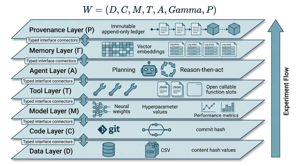
Mental Model
Think of the seven-layer workbench as a professional kitchen preparing a complex dish. The Memory Layer is the head chef's experience (remembering which techniques worked on similar dishes). Data, Code, and Models are the pantry, the recipe book, and the pre-made stocks: raw ingredients, instructions, and prepared components that feed into execution. The Tool Layer is the set of kitchen equipment (ovens, mixers, thermometers) that actually transforms ingredients. The Agent Layer is the sous-chef who reads the recipe, pulls the right ingredients, picks the right equipment, and sequences every step. The Provenance Layer is the kitchen's log book, recording exactly which batch of flour went into which loaf, at what temperature, for how long. The key mapping: just as a sous-chef who forgets to check the log book might reuse a contaminated batch, an agent that bypasses provenance produces results no one can verify.
Each layer exists because removing it causes a specific, predictable failure mode:
- No Data Layer: Datasets mutate silently. You cannot determine whether a result changed because of your code or because the training data was updated.
- No Code Layer: You cannot reproduce a result because you do not know which version of the code generated it.
- No Model Layer: Trained models are lost, overwritten, or impossible to associate with their training conditions.
- No Tool Layer: Agents cannot act on the world. The system can think but not do.
- No Agent Layer: Every experiment requires manual orchestration. The system scales with human attention, which does not scale.
- No Memory Layer: The system repeats failed experiments and forgets successful strategies. Every run starts from zero context.
- No Provenance Layer: Results exist but cannot be trusted, explained, or reproduced. Science without provenance is anecdote.
Research Frontier
The layered workbench pattern described here treats each layer as a static, human-designed contract. Recent work pushes toward systems where agents themselves propose and modify the architecture. In 2025, Huang et al. introduced MLR-Copilot ("Autonomous Machine Learning Research," NeurIPS 2024 workshop; full system described in their 2025 arXiv preprint), a framework in which an LLM agent autonomously generates research hypotheses, writes experiment code, executes runs, and iterates on results, effectively acting as its own Code, Tool, and Agent Layers simultaneously. More radically, Sakana AI's "The AI Scientist" (2024) demonstrated end-to-end paper generation from idea to LaTeX write-up, revealing both the promise and the failure modes (fabricated metrics, uncaught errors) that emerge when provenance and memory layers are underspecified. These systems validate the seven-layer decomposition by showing precisely what breaks when layers are merged or omitted in autonomous pipelines.
10. Putting It Together: The Workbench Registry
The complete workbench is a composite object that holds references to all seven layers and provides a unified interface for running experiments. Here is a minimal but functional implementation:
from dataclasses import dataclass, field
from pathlib import Path
from typing import Any
from uuid import UUID


@dataclass
class ExperimentSpec:
    """What an agent submits to run an experiment."""
    hypothesis: str
    dataset_id: UUID
    code_commit: str
    tool_sequence: list[str]
    parameters: dict[str, Any] = field(default_factory=dict)
    budget_usd: float = 10.0
    max_steps: int = 100


@dataclass
class ExperimentResult:
    """What the workbench returns after an experiment completes."""
    run_id: UUID
    status: str                         # "completed" | "failed" | "budget_exceeded"
    outputs: dict[str, Any] = field(default_factory=dict)
    metrics: dict[str, float] = field(default_factory=dict)
    provenance_ids: list[UUID] = field(default_factory=list)
    cost_usd: float = 0.0


class DiscoveryWorkbench:
    """Top-level orchestrator that composes all seven layers."""

    def __init__(
        self,
        data: DataLayer,
        tool: ToolLayer,
        storage_root: Path = Path("./workbench"),
    ):
        self.data = data
        self.tool = tool
        self._storage = storage_root
        self._runs: dict[UUID, ExperimentResult] = {}

    def run_experiment(self, spec: ExperimentSpec) -> ExperimentResult:
        """Execute a full experiment through all seven layers."""
        from uuid import uuid4

        run_id = uuid4()
        provenance_chain: list[UUID] = []
        total_cost = 0.0

        # 1. Retrieve dataset (Data Layer)
        dataset = self.data.retrieve(spec.dataset_id)
        provenance_chain.append(dataset.id)

        # 2. Verify code commit (Code Layer, simplified)
        # In production: check git status, refuse dirty trees
        assert len(spec.code_commit) == 40, "Provide a full SHA-1 commit hash."
        provenance_chain.append(uuid4())  # code snapshot ID

        # 3. Execute tool sequence (Tool + Model Layers)
        outputs: dict[str, Any] = {}
        for tool_name in spec.tool_sequence:
            if total_cost >= spec.budget_usd:
                return ExperimentResult(
                    run_id=run_id,
                    status="budget_exceeded",
                    cost_usd=total_cost,
                    provenance_ids=provenance_chain,
                )
            result = self.tool.invoke(tool_name, spec.parameters)
            outputs[tool_name] = result["result"]
            total_cost += result.get("cost_usd", 0.0)
            provenance_chain.append(uuid4())

        # 4. Record result (Provenance Layer)
        experiment_result = ExperimentResult(
            run_id=run_id,
            status="completed",
            outputs=outputs,
            provenance_ids=provenance_chain,
            cost_usd=total_cost,
        )
        self._runs[run_id] = experiment_result
return experiment_resultDiscoveryWorkbench.run_experiment() composing Data, Code, Tool, and Provenance Layers into a single execution path with budget enforcement and provenance-chain construction. Section 6.4 extends this skeleton with SQLite-backed persistence and a FastAPI endpoint.Listing 6.4 is deliberately incomplete: it covers four layers (Data, Code, Tool, Provenance) and leaves Agent and Memory for later chapters. The architecture supports incremental extension. Adding the Memory Layer should not require changes to the Data Layer; adding a new agent type should not require changes to the Tool Layer. If modifying layer \(X\) forces a change in layer \(Y\), the boundary between them is wrong.
Try It: Build a Two-Layer Workbench in 30 Minutes
Stand up a minimal Data Layer and Provenance Layer on your laptop to experience the architecture firsthand. You need only Python 3.10+ and the standard library.
- Create a project folder with two subdirectories:
data_store/(for registered datasets) andprovenance/(for JSON log files). Place a small CSV file (any tabular data with at least two columns) indata_store/. - Implement the Data Layer. Copy the
DatasetandDataLayerclasses from Listing 6.2 into a file calledworkbench.py. Register your CSV file, then retrieve it and print the content hash. Verify that modifying even a single byte in the CSV causesretrieve()to raise aValueError. - Add a provenance log. After each
register()andretrieve()call, append a JSON record toprovenance/log.jsonlcontaining the action name, artifact ID, timestamp (datetime.utcnow().isoformat()), and the content hash. Usejson.dumps()and plain file I/O. - Simulate a versioning scenario. Add a new row to your CSV, re-register it under the same name but with
version=2, and confirm that both versions appear in your provenance log with distinct content hashes. - Query the provenance log. Write a function that, given an artifact ID, reads
log.jsonland returns every action ever performed on that artifact, sorted by timestamp. Run it and inspect the output to see the full history of your dataset.
By the end, you will have a working (if minimal) system that enforces data integrity and records provenance. This skeleton is exactly what the full DiscoveryWorkbench in Listing 6.4 builds on.
Exercise 6.1.1
The WorkbenchLayer base class in Listing 6.1 defines four abstract methods. Suppose you add a new layer called the Constraint Layer, responsible for storing safety constraints that agents must obey (for example, "never exceed 500 K reaction temperature" or "do not call tools costing more than \$5 without approval"). Write the class signature for a ConstraintLayer(WorkbenchLayer) that implements the four base methods and adds one domain-specific method, check(action: dict) -> bool, which returns True if a proposed action satisfies all registered constraints. Which of the seven existing layers should the Constraint Layer sit between, and why?
Hint
The Constraint Layer logically sits between the Agent Layer and the Tool Layer: the agent proposes an action, the constraint check runs, and only passing actions reach the Tool Layer for execution. For the four base methods, think of each constraint as aLayerArtifact with a unique ID, a version (constraints evolve), and lineage back to the policy document or regulatory source that motivated it.Step-Through: An Experiment Traverses All Seven Layers
Trace through a single experiment run using the DiscoveryWorkbench.run_experiment() from Listing 6.4 with these concrete values:
- Memory Layer (query): the agent asks "any prior DFT runs on methane with B3LYP?" and retrieves one memory entry with cosine similarity 0.91, which notes that the 6-31G* basis set converged in 12 minutes for similar hydrocarbons.
- Data Layer (retrieve): the agent loads dataset
ds-0042(methane geometry XYZ file, 5 atoms, content hasha3f7c1...). The SHA-256 check passes. - Code Layer (verify): Git commit
e9b2d4f...is checked; the working tree is clean, so registration proceeds. - Tool Layer (invoke): the agent calls
run_dft_calculationwithgeometry_xyz="CH4.xyz",functional="B3LYP",basis_set="6-31G*". The tool returns{"energy_hartree": -40.5184, "converged": true}. Cost: \$2.50. - Model Layer (store): no model is trained in this run, so this layer is untouched.
- Memory Layer (write): the agent stores a new entry: "B3LYP/6-31G* on methane converged, energy = -40.5184 Ha, cost \$2.50, runtime 9 min."
- Provenance Layer (record): a chain of four UUIDs is written, linking
ds-0042to commite9b2d4fto the DFT tool invocation to the final result, with timestamps at each step.
Notice that seven layers were touched even for a single, simple calculation. The Model Layer was skipped because no training occurred, but it remained available. The total cost returned is \$2.50, and the status is "completed".
Real-World Application: Google DeepMind's GNoME
Google DeepMind's GNoME (Graph Networks for Materials Exploration) system, which predicted over 2.2 million stable crystal structures in 2023, effectively implements analogues of all seven workbench layers at industrial scale. Its Data Layer manages the Materials Project and ICSD crystallographic databases (millions of entries, each versioned and hashed). Its Agent Layer runs autonomous exploration loops that propose candidate structures, invoke DFT simulation tools, evaluate stability with trained graph neural network models, and record every decision in a provenance graph. The Memory Layer retains prior stability predictions so the agent avoids re-exploring known unstable regions of composition space.
The Trench Coat Was Always YAML
The epigraph's joke about microservices in a trench coat has a real ancestor. In 1968, Edsger Dijkstra published "The Structure of the THE Multiprogramming System," one of the first descriptions of layered software architecture. His system had six layers, not seven, and ran on an Electrologica X8 with 32 KB of memory. Dijkstra's key insight was identical to ours: each layer should be testable in isolation, with higher layers depending only on the contracts of lower ones. The THE system's "trench coat" was punched cards, not YAML, but the principle that good layer boundaries prevent cascading failures has not changed in nearly sixty years.
Lab: Build and Break a Three-Layer Workbench
Goal: Experience firsthand what breaks when a workbench layer is missing or bypassed.
Tools needed: Python 3.10+, the standard library (no external packages), and a text editor.
Setup (5 minutes): Copy the LayerArtifact, WorkbenchLayer, Dataset, DataLayer, ToolSpec, and ToolLayer classes from Listings 6.1 through 6.3 into a single file. Create a small CSV with three columns and five rows.
Experiment 1, Integrity (10 minutes): Register the CSV, retrieve it, and confirm the hash check passes. Then open the CSV, change one value, and call retrieve() again. Observe the ValueError. Now remove the hash check from retrieve() (comment out the verification block) and repeat. Notice that the silent corruption goes undetected. Restore the check.
Experiment 2, Provenance (10 minutes): Add a simple provenance list that appends a dictionary ({"action": ..., "artifact_id": ..., "timestamp": ...}) after every register() and retrieve(). Run three register/retrieve cycles, then query the provenance list for one artifact ID. Now delete the provenance list and repeat. Try to answer: "Which version of the dataset did experiment 2 use?" without provenance.
What to observe: The gap between "I know what I did" (when you just ran it) and "I can prove what I did" (when provenance is present) becomes vivid within minutes, not months.
Exercises
- Conceptual: Consider a genomics lab that runs CRISPR screening experiments. Map each of the seven workbench layers to a concrete component in their workflow. For example, the Data Layer might correspond to their FASTQ file archive. What serves as their Memory Layer? Their Provenance Layer?
- Coding: Extend the
DataLayerin Listing 6.2 to support versioning. When a dataset with the same name but different content hash is registered, it should create a new version rather than raising an error. Implementlist_versions()to return all versions of a named dataset, sorted by creation time. - Analysis: Pick two open-source ML experiment tracking platforms (e.g., MLflow, Weights & Biases, Neptune, DVC). For each, identify which of the seven layers it covers natively, which it covers partially, and which it does not address at all. Present your findings as a \(7 \times 2\) coverage matrix with entries from {full, partial, none}.
- Design: Suppose you remove the Provenance Layer from the workbench. Write a one-paragraph scenario describing a specific, concrete failure that would result six months later when a reviewer questions one of your published results. Be precise about what information would be missing and why it matters.
What's Next
We have defined the seven layers and their contracts, but we have not yet addressed how artifacts within and across layers are connected. In Section 6.2: Artifact Graphs and Provenance, we formalize the workbench as a directed acyclic graph where nodes are artifacts and edges are derivation relationships. We will build the run record schema, implement human-in-the-loop approval gates, and show how to answer the question "where did this result come from?" in constant time.
Bibliography
The influential argument that in many domains, more data beats better algorithms, motivating the Data Layer as a first-class architectural concern.
Introduced MLflow's design for tracking experiments, packaging code, and managing model versions, directly inspiring the Model Layer contract in this chapter.
The W3C standard for representing provenance information, defining the entity-activity-agent model used by our Provenance Layer.
Demonstrated an LLM-driven agent that autonomously plans and executes chemistry experiments, exemplifying the Agent and Tool Layers working in concert.
Showed that language models can learn when and how to invoke external tools, providing the conceptual foundation for the Tool Layer's agent-facing catalog.
The open-source tool for versioning datasets and ML pipelines alongside Git, implementing many Data Layer and Code Layer contracts described in this section.
Introduced memory architectures for LLM-based agents (reflection, retrieval, planning), directly informing the Memory Layer's design in this chapter.
The foundational RAG paper, establishing the embed-retrieve-generate pattern that underlies the Memory Layer's semantic recall mechanism.
Google DeepMind's GNoME system, a real-world example of all seven layers operating at scale: massive crystallographic data, versioned models, autonomous agent loops, and full provenance.
The widely adopted framework for composing LLM agents with tools and memory, providing production implementations of the Agent, Tool, and Memory Layer patterns. As of 2025, LangGraph (the graph-based agent orchestration layer built on top of LangChain) has become the recommended approach for stateful, multi-step agent workflows, superseding LangChain's earlier sequential chain abstractions.