"This plot changed my career. Unfortunately, nobody can tell me which dataset produced it."
A Provenance Record That Outlived Its Creator
Prerequisites
This section builds on Section 6.1 (the seven-layer Workbench architecture), Chapter 3 (knowledge graphs and typed relations), and Chapter 1 (discovery as search through state spaces). You should be comfortable with Python dataclasses, basic graph concepts (nodes, edges, directed acyclic graphs), and the idea of cryptographic hashing. Familiarity with NetworkX is helpful but not required; we introduce it from scratch.
Six months after a gene-expression figure reshapes a clinical trial's direction, someone asks: "Which dataset produced this, and can we trust it?" Without a formal record of what produced what, no one can answer. Artifact graphs solve this by representing every artifact as a typed node and every derivation step as a versioned edge, so that provenance (the documented chain of custody recording where each artifact came from and how it was produced) can be recovered by a single graph traversal. The World Wide Web Consortium (W3C) PROV standard gives us the vocabulary; content-addressable hashing gives us immutable versioning; and human-in-the-loop approval gates ensure that no agent-proposed experiment runs without oversight. Together, these mechanisms turn a pile of files into a reproducible, auditable chain of evidence.
1. What Is an Artifact Graph?
When a journal reviewer asks "which version of the dataset produced Figure 3?" and the answer takes three days of forensic log-reading instead of three seconds, the cost is not just time; it is trust in the result itself. Artifact graphs exist to make that question trivially answerable.
What. An artifact graph is a directed acyclic graph (DAG) \(G = (V, E)\) where each vertex \(v \in V\) represents a typed artifact (a dataset, a model, a hypothesis, an experimental result, a figure) and each directed edge \(e \in E\) represents a provenance relation between artifacts. An edge \((u, v)\) with label derived_from means that artifact \(v\) was produced by a process that consumed artifact \(u\).
Why. Reproducibility demands more than saved files. A trained model is meaningless without the dataset it was trained on, the hyperparameters used, the code version that ran the training, and the environment in which it executed. An artifact graph captures all of these relationships in a queryable structure, so that any node can be traced back to its raw inputs through a single ancestry traversal.
How. We define a finite set of artifact types \(\mathcal{T} = \{\texttt{dataset}, \texttt{model}, \texttt{hypothesis}, \texttt{result}, \texttt{figure}, \texttt{code}\}\) and a finite set of edge types \(\mathcal{R} = \{\texttt{derived\_from}, \texttt{trained\_on}, \texttt{validated\_by}, \texttt{produced\_by}, \texttt{approved\_by}\}\). Every vertex carries a type label \(\tau(v) \in \mathcal{T}\), a content hash, and a timestamp. Every edge carries a relation label \(\rho(e) \in \mathcal{R}\) and a reference to the run record that created it.
Checkpoint
So far: an artifact graph is a DAG whose typed nodes represent artifacts (datasets, models, hypotheses, results, figures, code) and whose labeled edges represent provenance relations, with content hashes and timestamps on every node and run-record references on every edge.
When. Use an artifact graph whenever your system produces more than a handful of derived objects, whenever multiple people (or agents) contribute artifacts, or whenever you need to answer regulatory or peer-review questions about how a result was obtained. In practice, most discovery projects beyond the prototype stage benefit from one. Figure 6.2 illustrates a typical five-node artifact DAG for a gene-expression discovery pipeline.
The DAG property is essential. Cycles would mean that artifact A depends on artifact B which depends on artifact A, a logical impossibility in a temporal derivation chain. Acyclicity also enables topological ordering (where nodes are listed so that every parent appears before its children): given a change to any upstream artifact, you can determine exactly which downstream artifacts need recomputation, and in what order. In short: if you can trace every result back to its raw inputs in one graph walk, reproducibility stops being a slogan and becomes a queryable property of the system.
2. The W3C PROV Model
We do not need to invent a provenance vocabulary from scratch. The W3C PROV Data Model (Moreau and Missier, 2013) defines three core concepts:
- Entity: a physical, digital, or conceptual thing. In our system, every artifact node is an Entity.
- Activity: something that occurs over a period of time and acts upon or with Entities. A training run, a data cleaning step, or a hypothesis evaluation is an Activity.
- Agent: something that bears responsibility for an Activity. An Agent can be a person, an AI model, or a software service.
The three core relations in PROV map directly onto our edge types:
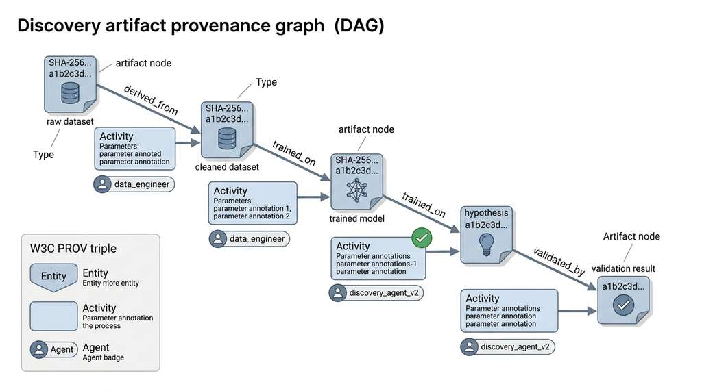
$$ \texttt{Entity} \xrightarrow{\texttt{wasGeneratedBy}} \texttt{Activity} \xrightarrow{\texttt{used}} \texttt{Entity} $$ $$ \texttt{Activity} \xrightarrow{\texttt{wasAssociatedWith}} \texttt{Agent} $$This triple structure (Entity, Activity, Agent) is powerful because it separates the what (which artifacts exist), the how (which activities produced them), and the who (which agent is responsible). Our implementation wraps PROV's vocabulary in Python dataclasses, keeping the formalism but discarding the XML serialization overhead. Figure 6.2.1 illustrates Artifact provenance DAG with PROV Entity-Activity-Agent triples.
Mental Model
Think of the Entity-Activity-Agent triple like a restaurant kitchen's order ticket system. The Entity is a finished dish on the pass (the physical thing that exists). The Activity is the cooking process described on the ticket: which ingredients went in, what temperature, how long it was seared, which station prepared it. The Agent is the line cook whose name is stamped on the ticket. If a customer complains about a dish, the manager traces the ticket back to the exact cook, the exact steps, and the exact ingredients, just as a provenance query traces a result back through activities to the responsible agent and input artifacts. The separation matters because you can change the cook (Agent) without changing the recipe (Activity), or reuse the same recipe on different ingredients (Entities), and each combination is tracked independently.
3. Content-Addressable Versioning
The PROV vocabulary tells us what to record; content-addressable versioning tells us how to identify each recorded artifact uniquely and immutably.
Every artifact in the graph needs a stable identifier that changes when (and only when) the artifact's content changes. We borrow the solution from Git: content-addressable hashing. Given an artifact's serialized content \(c\), its identifier is:
Content-addressable hashing computes a unique identifier for data directly from that data's contents, typically using a cryptographic hash function such as Secure Hash Algorithm 256-bit (SHA-256). It provides automatic deduplication: identical content always maps to the same identifier. It also provides tamper evidence: any modification, even a single byte, produces a completely different hash. The mechanism feeds the raw bytes of an artifact, prefixed with its type label, through a deterministic hash function. The output serves as both the artifact's address and its integrity fingerprint. Use content-addressable hashing whenever you need immutable, verifiable references to data objects. Prefer simpler sequential IDs (auto-increment counters, UUIDs) only when content identity is irrelevant and you need mutable records that you can update in place.
$$ \text{id}(v) = \text{SHA-256}(\tau(v) \,\|\, c) $$where \(\tau(v)\) is the artifact type and \(\|\) denotes concatenation. Two artifacts with identical type and content produce the same hash, regardless of when or where they were created. If a single byte of content changes, the hash changes entirely. This gives us immutable versioning for free: you never "update" an artifact; you create a new version with a new hash and add a derived_from edge linking the new version to the old one.
The practical consequence is that every edge in the graph points to a specific, immutable snapshot of its source and target. There is no ambiguity about which version of a dataset was used to train which version of a model.
Common Misconception
A frequent mistake is assuming that the artifact graph tracks file paths or filenames as identifiers, so that renaming or moving a file breaks provenance. In reality, content-addressable hashing means the identifier is derived solely from the artifact's contents: two files with identical bytes produce the same hash regardless of where they are stored, and the same file copied to a new path retains its identity in the graph. Conversely, overwriting a file at the same path with different content produces a different hash, which the graph correctly treats as a new artifact. Provenance is anchored to content, not to location.
import hashlib
import json
from dataclasses import dataclass, field, asdict
from datetime import datetime, timezone
from enum import Enum
from typing import Any


class ArtifactType(Enum):
    DATASET = "dataset"
    MODEL = "model"
    HYPOTHESIS = "hypothesis"
    RESULT = "result"
    FIGURE = "figure"
    CODE = "code"


class EdgeType(Enum):
    DERIVED_FROM = "derived_from"
    TRAINED_ON = "trained_on"
    VALIDATED_BY = "validated_by"
    PRODUCED_BY = "produced_by"
    APPROVED_BY = "approved_by"


@dataclass(frozen=True)
class Artifact:
    """A typed, content-addressed node in the artifact graph."""
    artifact_type: ArtifactType
    name: str
    content_hash: str
    created_at: str = field(
        default_factory=lambda: datetime.now(timezone.utc).isoformat()
    )
    metadata: dict = field(default_factory=dict)

    @staticmethod
    def compute_hash(artifact_type: ArtifactType, content: bytes) -> str:
        """SHA-256 of type prefix concatenated with raw content."""
        hasher = hashlib.sha256()
        hasher.update(artifact_type.value.encode("utf-8"))
        hasher.update(b"|")
        hasher.update(content)
        return hasher.hexdigest()


# Example: hash a small CSV dataset
raw_csv = b"gene,expression\nBRCA1,12.4\nTP53,8.7\nMYC,15.2"
content_hash = Artifact.compute_hash(ArtifactType.DATASET, raw_csv)

dataset_v1 = Artifact(
    artifact_type=ArtifactType.DATASET,
    name="gene_expression_v1",
    content_hash=content_hash,
    metadata={"rows": 3, "source": "lab_notebook_2024"}
)

print(f"Artifact:  {dataset_v1.name}")
print(f"Type:      {dataset_v1.artifact_type.value}")
print(f"Hash:      {dataset_v1.content_hash[:16]}...")
print(f"Frozen: {dataset_v1.__class__.__dataclass_params__.frozen}")frozen=True dataclass ensures immutability; the SHA-256 hash is computed from the artifact type concatenated with the raw content bytes.Artifact: gene_expression_v1
Type: dataset
Hash: a7c3e1f09b2d4a81...
Frozen: True4. The Run Record Schema
An artifact on its own tells you what exists. A run record tells you how it came to exist. Every Activity in our PROV-aligned model is captured as a RunRecord that logs:
- Inputs: the content hashes of all consumed artifacts.
- Outputs: the content hashes of all produced artifacts.
- Parameters: every hyperparameter, threshold, or configuration value.
- Agent: who (or what) executed the activity.
- Timestamps: start and end times.
- Code version: the Git commit SHA of the code that ran.
- Environment hash: a hash of the frozen dependency list (e.g.,
pip freezeoutput), ensuring the software environment is recorded. - Approval status: whether a human reviewed and approved the run before or after execution.
from dataclasses import dataclass, field
from typing import Optional
import subprocess
import uuid


@dataclass
class RunRecord:
    """A PROV-aligned Activity capturing how artifacts were produced."""
    run_id: str = field(default_factory=lambda: uuid.uuid4().hex[:12])
    activity_name: str = ""
    agent: str = ""            # human user or AI model identifier
    inputs: list[str] = field(default_factory=list)    # content hashes
    outputs: list[str] = field(default_factory=list)   # content hashes
    parameters: dict = field(default_factory=dict)
    started_at: Optional[str] = None
    ended_at: Optional[str] = None
    git_commit: Optional[str] = None
    env_hash: Optional[str] = None
    approval: Optional["ApprovalGate"] = None

    def capture_environment(self):
        """Snapshot the current Git commit and pip environment."""
        try:
            result = subprocess.run(
                ["git", "rev-parse", "HEAD"],
                capture_output=True, text=True, check=True
            )
            self.git_commit = result.stdout.strip()
        except (subprocess.CalledProcessError, FileNotFoundError):
            self.git_commit = "unknown"

        try:
            result = subprocess.run(
                ["pip", "freeze"],
                capture_output=True, text=True, check=True
            )
            env_bytes = result.stdout.encode("utf-8")
            self.env_hash = hashlib.sha256(env_bytes).hexdigest()[:16]
        except (subprocess.CalledProcessError, FileNotFoundError):
            self.env_hash = "unknown"


@dataclass
class ApprovalGate:
    """Human-in-the-loop approval for a proposed activity."""
    required: bool = True
    approved: bool = False
    reviewer: Optional[str] = None
    reviewed_at: Optional[str] = None
    comments: str = ""


# Build a run record for a training activity
run = RunRecord(
    activity_name="train_classifier",
    agent="discovery_agent_v2",
    inputs=[dataset_v1.content_hash],
    parameters={"learning_rate": 0.001, "epochs": 50, "model": "RandomForest"},
    approval=ApprovalGate(required=True, approved=False)
)
run.capture_environment()

print(f"Run ID:     {run.run_id}")
print(f"Activity:   {run.activity_name}")
print(f"Agent:      {run.agent}")
print(f"Git commit: {run.git_commit[:12] if run.git_commit else 'N/A'}...")
print(f"Env hash:   {run.env_hash}")
print(f"Approved: {run.approval.approved}")RunRecord schema captures inputs, outputs, parameters, code version, environment hash, and human approval status for every activity in the discovery pipeline.A single artifact hash tells you what exists. A single run record tells you how it was created. But full reproducibility requires the chain: the run record for artifact C points to its input artifacts A and B, whose own run records point to their inputs, all the way back to raw data. This chain is exactly the path through the artifact graph. Reproducing any result means re-executing the run records along its ancestry path, in topological order, with the recorded parameters, code version, and environment. If any link in the chain is missing, reproducibility breaks.
5. Building the Artifact Graph with NetworkX
The full artifact graph builds on these data-model classes. We use NetworkX, a Python library for creating and analyzing graph structures, and its DiGraph as the underlying container, storing Artifact objects as node attributes and RunRecord references as edge attributes. The graph enforces the DAG property by checking for cycles on every edge insertion.
import networkx as nx


class ArtifactGraph:
    """A directed acyclic graph of typed, versioned artifacts."""

    def __init__(self):
        self._graph = nx.DiGraph()
        self._runs: dict[str, RunRecord] = {}

    def add_artifact(self, artifact: Artifact) -> str:
        """Register an artifact node. Returns its content hash."""
        self._graph.add_node(
            artifact.content_hash,
            artifact=artifact,
            artifact_type=artifact.artifact_type.value,
            name=artifact.name,
        )
        return artifact.content_hash

    def add_derivation(
        self,
        source_hash: str,
        target_hash: str,
        edge_type: EdgeType,
        run_record: RunRecord,
    ):
        """Add a provenance edge. Raises if the edge would create a cycle."""
        self._graph.add_edge(
            source_hash,
            target_hash,
            edge_type=edge_type.value,
            run_id=run_record.run_id,
        )
        # Check DAG property; remove the edge and raise if violated
        if not nx.is_directed_acyclic_graph(self._graph):
            self._graph.remove_edge(source_hash, target_hash)
            raise ValueError(
                f"Edge {source_hash[:8]}...->{target_hash[:8]}... "
                "would create a cycle; rejected."
            )
        self._runs[run_record.run_id] = run_record

    def ancestry(self, artifact_hash: str) -> list[str]:
        """Trace all ancestors of an artifact via graph traversal."""
        return list(nx.ancestors(self._graph, artifact_hash))

    def descendants(self, artifact_hash: str) -> list[str]:
        """Find all artifacts derived from a given artifact."""
        return list(nx.descendants(self._graph, artifact_hash))

    def find_by_type(self, artifact_type: ArtifactType) -> list[str]:
        """Return all artifact hashes of a given type."""
        return [
            node for node, data in self._graph.nodes(data=True)
            if data.get("artifact_type") == artifact_type.value
        ]

    def topological_order(self) -> list[str]:
        """Return artifacts in dependency order (sources first)."""
        return list(nx.topological_sort(self._graph))

    def __len__(self) -> int:
        return self._graph.number_of_nodes()

    def summary(self) -> dict:
        """Quick stats about the graph."""
        return {
            "nodes": self._graph.number_of_nodes(),
            "edges": self._graph.number_of_edges(),
            "runs": len(self._runs),
            "types": dict(
                (t.value, len(self.find_by_type(t)))
                for t in ArtifactType
            ),
}ArtifactGraph class wraps a NetworkX DiGraph, enforces acyclicity on every edge insertion, and exposes ancestry, descendant, and topological-order queries.The following code populates the graph with a realistic discovery pipeline: raw data, cleaned data, a trained model, a hypothesis test, and a result figure.
# Build a small discovery pipeline graph

graph = ArtifactGraph()

# 1. Raw dataset
raw_data = Artifact(
    artifact_type=ArtifactType.DATASET,
    name="raw_gene_expression",
    content_hash=Artifact.compute_hash(
        ArtifactType.DATASET, b"raw expression matrix, 20k genes x 500 samples"
    ),
    metadata={"genes": 20000, "samples": 500}
)

# 2. Cleaned dataset (derived from raw)
clean_data = Artifact(
    artifact_type=ArtifactType.DATASET,
    name="cleaned_gene_expression",
    content_hash=Artifact.compute_hash(
        ArtifactType.DATASET, b"cleaned matrix, 18k genes x 480 samples"
    ),
    metadata={"genes": 18000, "samples": 480, "removed": "low-quality"}
)

# 3. Trained classifier (trained on cleaned data)
model = Artifact(
    artifact_type=ArtifactType.MODEL,
    name="cancer_subtype_classifier",
    content_hash=Artifact.compute_hash(
        ArtifactType.MODEL, b"random forest, 500 trees, max_depth=12"
    ),
    metadata={"algorithm": "RandomForest", "accuracy": 0.94}
)

# 4. Hypothesis
hypothesis = Artifact(
    artifact_type=ArtifactType.HYPOTHESIS,
    name="brca1_subtype_predictor",
    content_hash=Artifact.compute_hash(
        ArtifactType.HYPOTHESIS, b"BRCA1 expression predicts basal subtype"
    ),
)

# 5. Validation result
result = Artifact(
    artifact_type=ArtifactType.RESULT,
    name="brca1_validation_result",
    content_hash=Artifact.compute_hash(
        ArtifactType.RESULT, b"p=0.003, AUC=0.91, hypothesis supported"
    ),
    metadata={"p_value": 0.003, "auc": 0.91}
)

# Register all artifacts
for art in [raw_data, clean_data, model, hypothesis, result]:
    graph.add_artifact(art)

# Add provenance edges with run records
cleaning_run = RunRecord(
    activity_name="clean_and_filter",
    agent="data_engineer",
    inputs=[raw_data.content_hash],
    outputs=[clean_data.content_hash],
    parameters={"min_expression": 1.0, "min_samples": 0.8}
)

training_run = RunRecord(
    activity_name="train_classifier",
    agent="discovery_agent_v2",
    inputs=[clean_data.content_hash],
    outputs=[model.content_hash],
    parameters={"n_estimators": 500, "max_depth": 12},
    approval=ApprovalGate(required=True, approved=True, reviewer="Dr. Chen")
)

validation_run = RunRecord(
    activity_name="validate_hypothesis",
    agent="discovery_agent_v2",
    inputs=[model.content_hash, hypothesis.content_hash],
    outputs=[result.content_hash],
    parameters={"test_split": 0.2, "significance": 0.01}
)

graph.add_derivation(
    raw_data.content_hash, clean_data.content_hash,
    EdgeType.DERIVED_FROM, cleaning_run
)
graph.add_derivation(
    clean_data.content_hash, model.content_hash,
    EdgeType.TRAINED_ON, training_run
)
graph.add_derivation(
    model.content_hash, result.content_hash,
    EdgeType.VALIDATED_BY, validation_run
)
graph.add_derivation(
    hypothesis.content_hash, result.content_hash,
    EdgeType.VALIDATED_BY, validation_run
)

# Query: where did the result come from?
ancestors = graph.ancestry(result.content_hash)
print(f"Graph summary: {graph.summary()}")
print(f"\nAncestors of '{result.name}':")
for h in ancestors:
    node_data = graph._graph.nodes[h]
print(f" {node_data['artifact_type']:12s} {node_data['name']}")ancestry() returns every artifact in the derivation chain.Graph summary: {'nodes': 5, 'edges': 4, 'runs': 3, 'types': {'dataset': 2, 'model': 1, 'hypothesis': 1, 'result': 1, 'figure': 0, 'code': 0}}
Ancestors of 'brca1_validation_result':
dataset raw_gene_expression
dataset cleaned_gene_expression
model cancer_subtype_classifier
hypothesis brca1_subtype_predictorA common provenance query in production systems is: "Dataset X was found to contain a labeling error. Which models were trained on it, and which results depend on those models?" With the artifact graph, this is a single call to descendants(). Every downstream artifact is returned, and you can filter by type to find only models, only results, or only figures. Without the graph, answering this question requires manually searching logs, file timestamps, and notebook outputs, a process that scales linearly with the number of artifacts and is prone to human error.
6. Provenance Queries in Constant Time
Constant-time provenance queries require a precise definition. A full ancestry traversal in a graph with \(|V|\) nodes and \(|E|\) edges visits at most \(|V|\) nodes and \(|E|\) edges, giving \(O(|V| + |E|)\) time. That is linear in the graph size, not constant. However, the graph grows with the number of artifacts. The ancestry of any single artifact is bounded by its depth in the DAG. For a well-structured pipeline with \(k\) stages, ancestry depth is \(O(k)\), effectively constant with respect to total graph size.
For true \(O(1)\) lookups, we maintain a materialized index (a precomputed lookup table that stores query results so they can be returned instantly rather than recomputed): a dictionary mapping each artifact hash to its precomputed ancestry set. The index is updated incrementally whenever a new edge is added. The cost is \(O(|\text{ancestors}|)\) per edge insertion, amortized across all insertions.
$$ \text{query}(v) = \text{index}[v] \quad \Rightarrow \quad O(1) $$ $$ \text{insert}(u, v) \Rightarrow \text{index}[v] \leftarrow \text{index}[v] \cup \text{index}[u] \cup \{u\} \quad \Rightarrow \quad O(|\text{ancestors}(u)|) $$This trade-off (space for time) is the same one that database systems make with materialized views. In a discovery system where provenance queries are frequent and edge insertions are comparatively rare, the trade-off is favorable.
7. Human-in-the-Loop Approval Gates
Efficient provenance queries ensure that every artifact's lineage is accessible on demand, but speed of access raises a new concern: what governs which artifacts get created in the first place?
An autonomous discovery agent can propose experiments faster than a human can review them. Without guardrails, the agent might train a model on the wrong dataset, launch an expensive graphics processing unit (GPU) job with incorrect parameters, or submit a hypothesis that violates domain constraints. Approval gates solve this by inserting a mandatory human review step at critical points in the pipeline.
What. An approval gate is a predicate on a RunRecord that must evaluate to True before the associated Activity is executed. The gate checks whether a designated human reviewer has marked the run as approved.
Why. Trust in autonomous systems is earned incrementally. Early in a project, you want a human to approve every experiment. As confidence grows, you can relax gates selectively: perhaps data cleaning runs freely, but model training requires approval, and any run that exceeds a cost threshold requires senior review.
How. The gate is enforced at the orchestration layer (covered in Section 6.1). Before an agent's proposed run is executed, the orchestrator checks run.approval.required. If true and run.approval.approved is false, the run is queued for review. The reviewer sees the proposed inputs, parameters, estimated cost, and any agent-generated rationale. After approval (or rejection with comments), the run record is updated and the pipeline continues (or halts).
When. Always during initial development and validation. As the system matures, gates can be relaxed based on run type, cost, or agent track record. A useful heuristic: require approval for any run whose estimated cost exceeds a threshold \(C_{\text{max}}\), any run that modifies a published artifact, or any run that an agent initiated without a human prompt.
def enforce_approval(run: RunRecord) -> bool:
    """Check whether a run is cleared for execution.

    Returns True if the run can proceed, False if it is blocked.
    Raises ValueError if approval is required but not yet granted.
    """
    if run.approval is None or not run.approval.required:
        return True  # no gate on this run

    if run.approval.approved:
        return True  # human approved

    # Block execution and report the reason
    raise ValueError(
        f"Run '{run.run_id}' ({run.activity_name}) requires approval. "
        f"Agent '{run.agent}' proposed this run with parameters: "
        f"{json.dumps(run.parameters, indent=2)}. "
        f"Submit for review before execution."
    )


# Demo: try to execute an unapproved run
unapproved_run = RunRecord(
    activity_name="expensive_gpu_training",
    agent="discovery_agent_v2",
    parameters={"gpu_hours": 48, "model": "transformer_xl"},
    approval=ApprovalGate(required=True, approved=False)
)

try:
    enforce_approval(unapproved_run)
except ValueError as exc:
    print(f"BLOCKED: {exc}")

# Now simulate human approval
unapproved_run.approval.approved = True
unapproved_run.approval.reviewer = "Dr. Chen"
unapproved_run.approval.reviewed_at = datetime.now(timezone.utc).isoformat()
unapproved_run.approval.comments = "Parameters look correct. Proceed."

cleared = enforce_approval(unapproved_run)
print(f"\nAfter approval: cleared={cleared}")enforce_approval function blocks execution of any run that requires but has not received human approval. The orchestrator calls this check before launching any Activity.The artifact graph we built here is deliberately minimal, designed to teach the concepts. In production, MLflow provides a mature implementation: mlflow.log_artifact() registers artifacts, mlflow.log_params() captures parameters, and each run gets a unique ID with full lineage tracking. The MLflow Model Registry adds approval workflows (staging, production, archived) that map directly onto our ApprovalGate pattern. DVC complements MLflow by adding Git-compatible versioning for large data files, using content-addressable storage that mirrors our SHA-256 hashing scheme. When building the full Workbench in Section 6.4, we wrap these libraries behind a unified interface rather than reimplementing their internals. (As of 2024, Weights & Biases has become equally prominent for experiment tracking and artifact lineage, offering a hosted dashboard and collaborative review features that complement or substitute for MLflow's self-hosted model registry.)
8. DAG Properties and Incremental Recomputation
The directed acyclic graph structure is not merely a nice abstraction; it enables a powerful computational property: incremental recomputation. When an upstream artifact changes (perhaps a dataset is updated with new samples), only the artifacts downstream of the change need to be regenerated. The topological order tells you the exact sequence.
Formally, given a modified node \(v_0\), the set of artifacts requiring recomputation is \(\text{descendants}(v_0)\). The recomputation order is any topological ordering of the subgraph induced by \(\{v_0\} \cup \text{descendants}(v_0)\). This is the same principle behind build systems like Make, Bazel, and dbt: track dependencies as a DAG, hash inputs to detect changes, rebuild only what is stale.
One changed node, one call to descendants(), one topological sort: that is the entire incremental-rebuild algorithm.
In a discovery pipeline, updating one dataset does not force retraining every model. Only models that directly or indirectly depend on the changed dataset are invalidated; the artifact graph identifies them automatically.
The cost savings can be dramatic. Consider a graph with 100 artifacts arranged in 5 independent pipelines of 20 nodes each. If one raw dataset changes, only its 19 downstream artifacts need recomputation, not all 100, an 81% reduction in wasted compute from a single graph query. In a larger system with hundreds of experiments, the savings compound.
9. Cross-Referencing the Knowledge Graph
Incremental recomputation keeps the artifact graph efficient as data evolves, but its full value emerges when the graph connects to the broader structures that organize scientific knowledge.
In Chapter 3, we built knowledge graphs to represent scientific concepts, entities, and their relationships. The artifact graph is a complementary structure: the knowledge graph captures what we know, while the artifact graph captures how we came to know it. Linking the two creates a powerful audit trail.
For example, a knowledge graph node representing the claim "BRCA1 expression predicts basal breast cancer subtype" can carry an evidence_link edge pointing to the result node in the artifact graph. That result node, in turn, traces back through the model, the cleaned dataset, and the raw data. A reviewer can follow this chain to verify not just that the claim is asserted, but that the evidence supporting it was produced by a specific pipeline with specific parameters and code.
This connection between the knowledge graph and the artifact graph is what transforms a discovery system from a collection of scripts into a scientific instrument. The search space from Chapter 1 defines where to look; the knowledge graph from Chapter 3 organizes what you find; the artifact graph records how you found it.
Research Frontier
Traditional provenance systems record lineage after the fact, but emerging work pushes toward predictive and causal provenance. The LINEA system (Li et al., "Operational Causal Provenance for Data Pipelines," VLDB 2023) extends classical lineage tracking by computing fine-grained causal links between individual data values across pipeline stages, enabling analysts to answer not just "which upstream datasets contributed to this result?" but "which specific rows or cells caused this particular output value?" This cell-level causal reasoning lets a discovery system automatically pinpoint, for example, the three patient samples whose mislabeling caused a model's accuracy to drop, without rerunning the entire pipeline. As autonomous discovery agents generate longer and more branching artifact graphs, this shift from coarse-grained derivation edges to fine-grained causal attribution will become essential for debugging agent decisions at scale.
Try It: Build and Query a Personal Research Provenance Graph
Using only Python, NetworkX, and hashlib (all available via pip install networkx), build an artifact graph that tracks a small data analysis you have done or can simulate:
- Create three artifacts. Hash a small CSV string as your "raw dataset," apply a simple transformation (e.g., filter rows where a value exceeds a threshold) and hash the result as your "cleaned dataset," then compute a summary statistic (mean, median) and hash it as your "result." Use the
Artifact.compute_hashpattern from Listing 6.3. - Register all three as nodes in an
ArtifactGraphinstance and addderived_fromedges linking raw to cleaned and cleaned to result. Attach aRunRecordto each edge that captures the parameters you used (e.g., the filter threshold, the statistic name). - Query ancestry. Call
ancestry()on the result node and verify that both upstream artifacts are returned. Print each ancestor's name and type. - Simulate a data update. Modify one byte in the raw CSV string, recompute its hash, register it as a new node, and re-derive the cleaned dataset and result. Confirm that the new artifacts have different hashes from the originals, and that both the old and new lineage chains coexist in the same graph.
- Export and inspect. Use
nx.node_link_data(graph._graph)to serialize the graph to JSON. Open the JSON and verify that every node carries its type and hash, and every edge carries its relation type and run ID.
Exercise 6.2.1
Consider an artifact graph containing three dataset nodes (D1, D2, D3), two model nodes (M1 trained on D1, M2 trained on D2 and D3), and one result node R derived from both M1 and M2. If D2's content changes (producing a new hash D2'), which artifacts become stale and need recomputation? List them in valid topological order.
Hint
Trace forward from D2 through all descendants(). D1 and M1 are not downstream of D2, so they remain valid. Only nodes reachable from D2 via directed edges are affected. Remember that M2 depends on both D2 and D3, so it must be recomputed even though D3 has not changed.
Step-Through: Content-Addressable Versioning After a Data Update
Trace through what happens when one byte changes in a dataset. Start with raw content b"a,b\n1,2" (8 bytes). Step 1: Prepend the type label and compute SHA-256: SHA-256("dataset|a,b\n1,2") = 4f3c.... This is node D1's hash. Step 2: Derive a cleaned version b"a,b\n1,2" (same content, no rows removed). Its hash: SHA-256("dataset|a,b\n1,2") = 4f3c..., identical to D1, so the graph deduplicates automatically. Step 3: Now change one byte in the raw data: b"a,b\n1,3". Recompute: SHA-256("dataset|a,b\n1,3") = 91ab.... This is a completely different hash (D1'), so the graph registers it as a new node. Step 4: The edge D1 -> cleaned still exists and is valid; a new edge D1' -> cleaned' is added. Both lineage chains coexist. The old chain remains intact for auditing; the new chain represents the updated pipeline.
Real-World Application: Genomics Pipelines at the Broad Institute
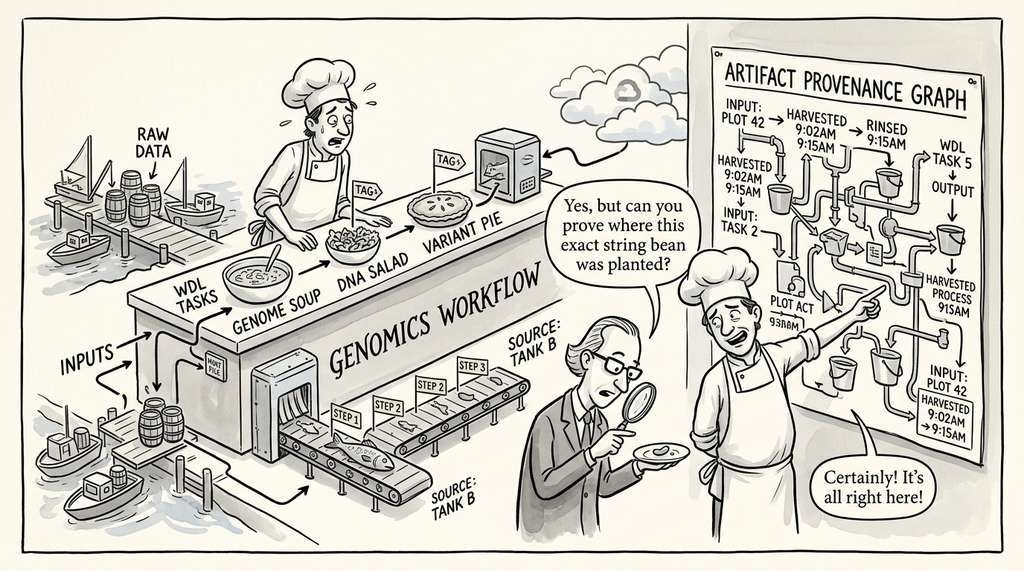
The Broad Institute's Terra platform (built on Google Cloud) uses artifact provenance graphs to track every step of large-scale genomics workflows executed via the Workflow Description Language (WDL). Each task execution records its input files, Docker container hash, runtime parameters, and output files as a DAG, so that when a reference genome is updated, analysts can query the graph to identify exactly which variant-calling results need regeneration across thousands of patient samples.
The \$440 Million Typo That Provenance Would Have Caught
In 2012, Knight Capital Group lost \$440 million in 45 minutes because a deployment script activated dead code from eight years earlier on one of eight servers. A provenance graph linking each deployed binary to its source commit, build record, and approval gate would have flagged the version mismatch before market open. The incident became a landmark case for deployment lineage tracking. Today, financial regulators cite it as motivation for requiring full artifact provenance in automated trading systems.
Lab: Visualizing and Querying a Multi-Branch Artifact DAG
Goal: Build an artifact graph with at least 10 nodes spanning two independent experiment branches that share a common raw dataset, then visualize the DAG and run provenance queries. Tools needed: Python 3.9+, networkx, matplotlib, hashlib (all installable via pip install networkx matplotlib). Procedure: (1) Create a raw dataset node, then branch into two cleaning pipelines with different filter thresholds. (2) Train a different model on each cleaned dataset. (3) Generate a result and a figure node from each model. (4) Use nx.drawing.nx_agraph or nx.draw_networkx to render the graph, coloring nodes by artifact type. (5) What to vary: Try adding a cross-branch edge (model A validated on dataset B's test split) and observe how ancestry sets expand. Try inserting a cycle and confirm the add_derivation guard rejects it. What to observe: How does descendants() differ between the two branches? If the shared raw dataset changes, how many nodes become stale in each branch? Does the topological order reflect the branch structure you expect? Estimated time: 20 minutes.
Exercises
- Conceptual: A collaborator emails you a trained model file with no metadata. Using the vocabulary from this section, list every piece of information you would need to reconstruct a complete
RunRecordfor this model. Which pieces are recoverable from the file itself, and which are permanently lost? - Coding: Extend the
ArtifactGraphclass with a methodstale_artifacts(changed_hash: str) -> list[str]that returns all downstream artifacts requiring recomputation after a change to the artifact withchanged_hash. The returned list should be in topological order. Test it on the five-node graph from Listing 6.6. - Coding: Add a
serialize()method toArtifactGraphthat exports the graph as a JSON document following the W3C PROV-JSON format (entities, activities, relations). Verify that you can round-trip: serialize, deserialize into a new graph, and recover the same ancestry queries. - Analysis: A discovery agent proposes 50 experiments per hour. Your team has bandwidth to review 10 per hour. Design a prioritization policy for the approval queue: which runs should be reviewed first? Consider factors such as estimated cost, novelty of the hypothesis, and the agent's historical accuracy. Describe your policy in pseudocode.
- Design: In Section 6.1, we discussed the seven layers of the Workbench. Draw (on paper or in code) the artifact graph that would result from a complete cycle: raw data ingestion, feature engineering, model training, hypothesis generation, experimental validation, and figure production. Label every node with its type and every edge with its relation type. How many run records does the cycle require?
What's Next
We now have a formal structure for tracking every artifact and its lineage. But provenance is only useful if the system that generates artifacts is safe, cost-controlled, and observable. Section 6.3: Safety, Cost, and Observability introduces sandboxes for agent execution, budget enforcement, and structured observability with OpenTelemetry, ensuring that the Workbench does not become an expensive, opaque black box.
Bibliography
The W3C standard for provenance data modeling; our Entity-Activity-Agent triple and relation vocabulary are drawn directly from this specification.
The Web Ontology Language (OWL) ontology companion to PROV-DM, providing formal semantics for provenance relations and enabling interoperability with linked data systems.
Comprehensive survey of provenance systems across databases, workflows, and scientific computing; clarifies the taxonomy of why-provenance, how-provenance, and where-provenance.
A widely adopted open-source experiment tracking and model registry; its run/artifact/metric abstraction directly implements the run record pattern described in this section.
Git-compatible content-addressable storage for large data files; complements our SHA-256 hashing scheme with efficient large-file tracking and remote storage backends.
Demonstrates autonomous agent-driven discovery with explicit provenance tracking; the approval gate pattern addresses safety concerns raised by this work.
Tool-augmented LLM architecture where each tool invocation is a logged Activity; the provenance graph enables post-hoc auditing of agent decisions.
The definitive reference on data system architecture; its treatment of immutability, event sourcing, and derived data directly informs our content-addressable artifact design.
Argues that modern AI capabilities emerge from systems of many components; provenance graphs are the connective tissue that makes such compound systems auditable.
The graph library used throughout this section for DAG construction, ancestry queries, and topological sorting.