Prerequisites
This section opens the chapter on AI scientists. You should be familiar with the four canonical research agent roles (literature, coding, analysis, reviewer) from Chapter 40, hypothesis generation techniques from Chapter 39, and the experiment design loop from Chapter 46. Familiarity with embedding spaces from Chapter 26 will help with the novelty detection material.
In Chapter 40, we built agents that handle individual research tasks: reading papers, writing code, running analysis, reviewing results. An AI scientist connects these agents into a closed loop that runs autonomously. This section formalizes what that loop looks like, defines the six phases every AI scientist system implements (whether explicitly or implicitly), and introduces the novelty filter that prevents the system from rediscovering known results. We also map out the autonomy spectrum, from copilot to fully autonomous, and explain why current systems cluster at one end.
1. The Six Phases of Automated Research
Imagine a system that, at 2 a.m. on a Tuesday, proposes a hypothesis no human suggested, writes the code to test it, trains a model, discovers the hypothesis fails, revises its own idea, and by sunrise has a publishable result on its fourth attempt, all without a single human keystroke. That is the automated research loop in action, and every AI scientist system, regardless of domain or architecture, implements some version of the same six-phase cycle that makes it possible.
Without an automated loop, a researcher's Tuesday hypothesis waits until Wednesday's implementation, Thursday's execution, and Friday's evaluation; by then, the original context has faded and the feedback arrives too late to steer the next idea. That lag between question and answer is the single largest bottleneck in empirical science.
An automated research loop is a software system that cycles through hypothesis generation, experimentation, and evaluation without waiting for human intervention between steps. It compresses days of sequential decision-making into hours of continuous compute, letting the system explore far more ideas per unit time.
The mechanism is straightforward: each phase produces a structured output (a hypothesis document, a code artifact, a results table, a review verdict) that feeds into the next phase. A controller routes failures back to earlier phases for revision. Use an automated loop rather than manual orchestration when experiments are cheap enough to tolerate discarded runs (under ~\$100 each) and when you can express the evaluation criteria programmatically. For expensive or subjective domains, the supervised variant (Level 2 in Section 4) is more appropriate. In short: close the loop so the machine never waits for a human to carry a result from one phase to the next.
The six phases are not a linear pipeline. Real research involves backtracking: a negative evaluation triggers a revised hypothesis; a critique reveals a flaw in the implementation; a report draft exposes gaps that require additional experiments. The most effective AI scientist architectures model research as a cyclic graph with conditional transitions, not as a waterfall. AI Scientist v2 (Section 53.2) makes this explicit with agentic tree search over the research space.
The six phases are:
- Propose. Generate a research hypothesis or idea. The input is a research domain, a set of existing results, and (optionally) a gap analysis from a knowledge graph. The output is a concrete, testable claim. In Chapter 39, we built hypothesis generators using structural hole detection (where structural holes are gaps in a knowledge graph where no edge connects two otherwise related clusters of concepts) and analogical transfer; those become the "propose" module here.
- Implement. Write the code needed to test the hypothesis. This includes data loading, model definition, training loops, evaluation metrics, and visualization. The coding agent from Section 40.1 handles this phase.
- Run. Execute the experiment. In machine learning (ML) research, this means training a model and recording metrics. In chemistry, it means sending instructions to lab hardware (Chapter 55). In mathematics, it means running a search algorithm over candidate solutions. The critical requirement is determinism: the same code and data must produce the same result.
- Evaluate. Analyze the experimental results. Compute statistical tests, compare against baselines, check for confounds. The analysis agent from Section 40.1 handles this, augmented with the causal reasoning tools from Chapter 31.
- Critique. Review the methodology and results for errors, biases, and weaknesses. This is the internal peer review step. The reviewer agent from Section 40.1 performs this, often implemented as a separate large language model (LLM) call with a critic prompt that incentivizes finding flaws rather than confirming success.
- Report. Write up the findings as a structured document (paper, technical report, or notebook). This phase also decides whether the result is worth reporting at all, or whether the loop should continue with a revised hypothesis.
Figure 53.1 shows the six-phase loop with its feedback edges.
2. Formalizing the Research Loop
We can express the research loop as a state machine. Let $S = \{s_{\text{propose}}, s_{\text{implement}}, s_{\text{run}}, s_{\text{evaluate}}, s_{\text{critique}}, s_{\text{report}}\}$ be the set of states, and let $T: S \times \{0, 1\} \to S$ be the transition function, where the binary input indicates success (1) or failure (0) at each phase. The key transitions on failure are:
$$ T(s_{\text{run}}, 0) = s_{\text{implement}} \quad \text{(code bug: fix and re-run)} $$ $$ T(s_{\text{evaluate}}, 0) = s_{\text{propose}} \quad \text{(null result: revise hypothesis)} $$ $$ T(s_{\text{critique}}, 0) = s_{\text{implement}} \quad \text{(methodological flaw: redesign)} $$On success, the transition is always to the next phase in sequence, with \(T(s_{\text{report}}, 1) = s_{\text{propose}}\) closing the loop for the next research idea. Each state is associated with a maximum retry count \(r_i\) that prevents infinite cycling. When the retry count is exhausted, the system either escalates to a human supervisor or abandons the current idea and moves to \(s_{\text{propose}}\).
Consider an AI scientist tasked with improving image classification on CIFAR-10 (a standard benchmark dataset of 60,000 tiny 32x32 color images across 10 categories). The propose phase generates the idea "applying mixup augmentation (a training technique that blends pairs of images and their labels to regularize the model) to a ViT will improve accuracy by 2%." The implement phase writes a PyTorch training script with Vision Transformer (ViT) and mixup. The run phase trains for 100 epochs (cost: ~\$3 on a cloud GPU). The evaluate phase computes test accuracy and compares against a baseline without mixup. If the improvement is statistically significant (\(p < 0.05\) on a paired t-test across 5 seeds), the critique phase checks for data leakage, proper cross-validation, and fair baseline comparison. If the critique passes, the report phase generates a LaTeX paper. Total wall-clock time: under 2 hours. Total cost: under \$15. This is precisely the workflow that AI Scientist v1 automates.
3. Novelty Detection Through Embedding Distance
The state machine above tells the loop when to keep iterating, but it says nothing about what is worth iterating on; without a filter, the system could cycle endlessly through ideas that duplicate published work.
An AI scientist that rediscovers known results wastes compute and, worse, could present existing knowledge as novel findings. Novelty detection is therefore a critical filter applied at the propose phase. The core idea is simple: embed the generated hypothesis in the same space as the existing literature, and reject hypotheses that are too close to published work.
Formalizing the Novelty Score
Let \(h\) be the text of a generated hypothesis, and let \(\mathcal{P} = \{p_1, p_2, \ldots, p_n\}\) be the set of existing papers in the relevant domain. We compute embeddings using a scientific text encoder \(\phi\) (such as SPECTER2, a transformer model trained on citation graphs to produce embeddings that capture scientific similarity, or a fine-tuned Sentence-BERT, a siamese network architecture that maps sentences to fixed-length vectors optimized for semantic comparison):
$$ \text{novelty}(h) = \min_{p_i \in \mathcal{P}} d(\phi(h), \phi(p_i)) $$where \(d\) is cosine distance. A hypothesis is accepted only if \(\text{novelty}(h) > \tau\), where \(\tau\) is a threshold calibrated on a held-out set of known-novel vs. known-derivative paper pairs. In practice, \(\tau \approx 0.3\) on cosine distance typically works well for ML research papers when using SPECTER2 embeddings, though the optimal value varies by subfield and corpus size. Figure 53.2 traces the decision flow from a candidate hypothesis through the novelty filter.
Mental Model
Think of the novelty filter as a plagiarism detector for ideas, not for text. Imagine you are pitching a new restaurant concept to investors. Before your meeting, you search every restaurant review site in the city: if an existing restaurant already serves the same cuisine, in the same format, to the same audience, your concept is "too close" and you need a new angle. The embedding distance is the measure of how different your menu is from every menu already out there. A small distance means someone already opened that restaurant; a large distance means you have found a genuine gap in the market. The threshold \(\tau\) is the investor's minimum novelty bar: below it, "we have seen this before"; above it, "tell me more."
The following implementation shows a novelty filter using SPECTER2 embeddings and a FAISS (Facebook AI Similarity Search) index for efficient nearest-neighbor search over a large corpus.
import numpy as np
import faiss
from transformers import AutoTokenizer, AutoModel
import torch


class NoveltyFilter:
    """Filter hypotheses by embedding distance to existing literature."""

    def __init__(
        self,
        model_name: str = "allenai/specter2",
        threshold: float = 0.3,
    ):
        self.tokenizer = AutoTokenizer.from_pretrained(model_name)
        self.model = AutoModel.from_pretrained(model_name)
        self.threshold = threshold
        self.index = None
        self.paper_ids: list[str] = []

    def _embed(self, texts: list[str]) -> np.ndarray:
        """Compute normalized embeddings for a batch of texts."""
        inputs = self.tokenizer(
            texts,
            padding=True,
            truncation=True,
            max_length=512,
            return_tensors="pt",
        )
        with torch.no_grad():
            outputs = self.model(**inputs)
        # Use CLS token embedding
        embeddings = outputs.last_hidden_state[:, 0, :]
        # L2-normalize for cosine similarity via inner product
        norms = torch.norm(embeddings, dim=1, keepdim=True)
        return (embeddings / norms).numpy()

    def build_index(
        self, papers: list[dict[str, str]]
    ) -> None:
        """Build FAISS index from existing papers.

        Each paper dict has 'id', 'title', and 'abstract' keys.
        """
        texts = [
            f"{p['title']}. {p['abstract']}" for p in papers
        ]
        embeddings = self._embed(texts)
        dim = embeddings.shape[1]
        self.index = faiss.IndexFlatIP(dim)  # inner product = cosine on normalized vecs
        self.index.add(embeddings)
        self.paper_ids = [p["id"] for p in papers]

    def check_novelty(
        self, hypothesis: str
    ) -> dict:
        """Check if a hypothesis is sufficiently novel.

        Returns dict with 'is_novel', 'distance', and
        'nearest_paper_id'.
        """
        embedding = self._embed([hypothesis])
        similarities, indices = self.index.search(embedding, k=1)
        # cosine distance = 1 - cosine similarity
        cosine_distance = 1.0 - similarities[0][0]
        nearest_id = self.paper_ids[indices[0][0]]
        return {
            "is_novel": cosine_distance > self.threshold,
            "distance": float(cosine_distance),
            "nearest_paper_id": nearest_id,
        }


# Usage
filter = NoveltyFilter(threshold=0.3)
filter.build_index(existing_papers)  # list of paper dicts

result = filter.check_novelty(
    "Applying spectral normalization to the attention weights "
    "of Vision Transformers reduces overfitting on small datasets "
    "by constraining the Lipschitz constant of each layer."
)
print(f"Novel: {result['is_novel']}, "
      f"Distance: {result['distance']:.3f}, "
      f"Nearest: {result['nearest_paper_id']}")
check_novelty method computes cosine distance between a hypothesis and the nearest existing paper; hypotheses below the threshold are rejected as insufficiently novel.
The novelty filter above uses raw embedding distance, which misses semantic nuances.
PaperQA2 provides
a higher-level alternative: ask the literature agent "Has this hypothesis been tested before?"
and let it search, retrieve, and synthesize an answer with citations. A single call to
paperqa.ask() replaces the embedding index with a retrieval-augmented answer
grounded in full paper texts. The tradeoff is cost (~\$0.10 per query vs. ~\$0.001 for
embedding lookup) and latency (~30 seconds vs. milliseconds). In practice, AI scientist
systems use the embedding filter as a fast first pass and PaperQA2 as a slower, more
accurate second pass for borderline cases.
4. The Autonomy Spectrum
AI scientist systems differ dramatically in how much autonomy they grant the AI. We can arrange them on a five-level spectrum (Table 53.1), analogous to the Society of Automotive Engineers (SAE) levels for autonomous driving. Figure 53.1.1 illustrates the autonomy spectrum for AI scientist systems.
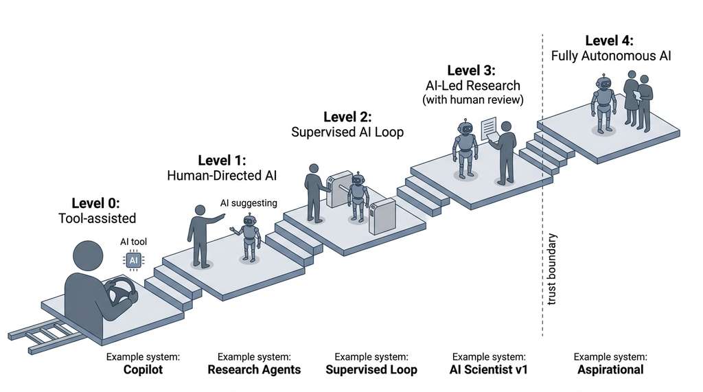
| Level | Name | Human Role | AI Role | Example |
|---|---|---|---|---|
| 0 | Tool-assisted | Drives every phase | Executes specific subtasks on request | GitHub Copilot |
| 1 | Copilot | Directs, approves each step | Suggests hypotheses, drafts code | Research agents (Ch 40) |
| 2 | Supervised | Approves at gates (hypothesis, experiment, report) | Runs the loop between gates | Section 53.4 recipe |
| 3 | Monitored | Reviews outputs post-hoc | Runs the full loop, flags anomalies | AI Scientist v1 |
| 4 | Fully autonomous | Sets the research agenda | Handles everything else | (Aspirational) |
Most current systems operate at Level 2 or 3. The barrier to Level 4 is largely institutional rather than purely technical: trust, safety, and accountability remain unsolved. A fully autonomous system risks burning compute on dead ends or, worse, generating plausible but wrong results that mislead downstream work. Level 2 balances throughput with human oversight.
Common Misconception
A frequent misconception is that "more autonomy is always better," that the goal is to push every AI scientist system to Level 4 as quickly as possible. In practice, higher autonomy increases the risk of compounding errors: a flawed hypothesis leads to a flawed experiment, which produces a flawed evaluation, which the system's own critic fails to catch because the critic shares the same blind spots as the proposer. Level 2 (supervised, with human gates at key decision points) currently produces higher quality research output than Level 3 systems precisely because human oversight catches failure modes that automated self-critique misses.
5. Why Current AI Scientists Are Domain-Limited
A striking pattern across all existing AI scientist systems is their confinement to domains where experiments are cheap, fast, and deterministic. AI Scientist v1 and v2 work on ML research, where an experiment costs a few dollars and completes in minutes. FunSearch works on discrete mathematics, where "experiments" are program evaluations that complete in milliseconds. Even Coscientist, which operates in the physical world, targets well-characterized reactions with predictable outcomes.
This limitation has three causes:
- Cost per experiment. An ML training run costs \$1 to \$100. A biology experiment costs \$1,000 to \$1,000,000. That is a cost gap of up to 10,000x, which is precisely why every current AI scientist system clusters in the cheap-experiment corner of the research landscape. An AI scientist that proposes and discards hundreds of ideas before finding one that works can only operate in low-cost domains.
- Feedback latency. ML experiments return results in minutes to hours. Wet-lab biology experiments take days to months. The research loop's iteration speed is bounded by the slowest phase, which is almost always the experiment execution.
- Determinism. Given the same code and data, an ML experiment produces the same result (modulo random seeds, which can be fixed). Biological experiments have intrinsic variability that makes automated evaluation harder. When the system cannot reliably distinguish "my hypothesis is wrong" from "the experiment had noise," the critique phase breaks down.
The path to AI scientists in expensive, slow, or noisy domains runs through simulation. Rather than executing a wet-lab experiment, the AI scientist runs a computational model of the experiment (see Chapter 43 and Chapter 44). Promising results from simulation are then forwarded to human experimentalists for physical validation. Google's AI Co-Scientist (Section 53.3) takes exactly this approach: it generates hypotheses computationally, then hands them to human scientists for wet-lab testing. The AI runs the cheap inner loop; humans run the expensive outer loop.
6. Measuring the Quality of Automated Research
Domain limitations constrain where AI scientists can operate today, but even within those domains we need a way to tell whether the research they produce is actually good.
How do you evaluate an AI scientist's output? The standard metrics from ML (accuracy, loss) do not apply. Instead, we need metrics specific to research quality. The following four dimensions, drawn from the evaluation framework of Huang et al. (2024), cover the space:
- Novelty. Is the finding genuinely new? Measured by embedding distance (Section 3 above) and expert assessment. Novelty without correctness is noise.
- Correctness. Are the experimental results valid? Measured by reproducibility: can an independent system re-run the experiment and obtain the same results? AI Scientist v1 reported ~70% reproducibility on its own generated experiments.
- Significance. Does the finding matter? Measured by effect size, statistical power, and expert assessment of impact. An AI scientist that discovers tiny improvements on saturated benchmarks produces correct but insignificant work.
- Clarity. Is the report well-written, well-structured, and easy to follow? Measured by automated readability metrics and (ideally) by human reviewers. AI Scientist v1's automated peer review scores its own papers on a 1-10 scale across multiple criteria.
We can combine these into a composite score with domain-specific weights:
$$ Q(r) = w_n \cdot \text{novelty}(r) + w_c \cdot \text{correctness}(r) + w_s \cdot \text{significance}(r) + w_l \cdot \text{clarity}(r) $$where \(r\) is a research output and \(w_n + w_c + w_s + w_l = 1\). In ML research, typical weights are \(w_c = 0.4\) (correctness dominates), \(w_n = 0.3\), \(w_s = 0.2\), \(w_l = 0.1\). The following code implements this evaluation framework.
from dataclasses import dataclass


@dataclass
class ResearchQuality:
    """Composite quality score for automated research output."""
    novelty: float       # 0-1: embedding distance score
    correctness: float   # 0-1: reproducibility fraction
    significance: float  # 0-1: effect size / expert rating
    clarity: float       # 0-1: readability + structure score

    def composite(
        self,
        weights: dict[str, float] | None = None,
    ) -> float:
        """Weighted composite score.

        Default weights emphasize correctness for ML research.
        """
        w = weights or {
            "novelty": 0.3,
            "correctness": 0.4,
            "significance": 0.2,
            "clarity": 0.1,
        }
        return (
            w["novelty"] * self.novelty
            + w["correctness"] * self.correctness
            + w["significance"] * self.significance
            + w["clarity"] * self.clarity
        )


def evaluate_reproducibility(
    experiment_fn,
    n_replications: int = 5,
    tolerance: float = 0.02,
) -> float:
    """Run an experiment multiple times and measure consistency.

    Returns fraction of replications within tolerance of the
    median result.
    """
    results = [experiment_fn(seed=i) for i in range(n_replications)]
    median_result = sorted(results)[n_replications // 2]
    within_tolerance = sum(
        1
        for r in results
        if abs(r - median_result) <= tolerance
    )
    return within_tolerance / n_replications


# Example usage
quality = ResearchQuality(
    novelty=0.72,       # moderately novel
    correctness=0.95,   # highly reproducible
    significance=0.45,  # modest improvement
    clarity=0.80,       # well-written
)
print(f"Composite quality: {quality.composite():.3f}")
# Output: Composite quality: 0.676
evaluate_reproducibility function measures correctness by running an experiment multiple times and checking consistency.To set the threshold \(\tau\) for the novelty filter, you need positive and negative examples. Collect 50 pairs of papers where one is the original contribution and the other is a follow-up that makes incremental changes (same method, different dataset). Compute the embedding distance for each pair: the distribution of these distances gives you the "derivative work" range, typically \([0.05, 0.25]\) for SPECTER2. Then collect 50 pairs of papers from different subfields that address unrelated problems. Their distances will cluster in \([0.4, 0.8]\). Set \(\tau\) at the decision boundary that maximizes separation, typically around 0.3. This calibration step takes about an hour of manual paper selection and a few minutes of compute.
7. From Research Agents to AI Scientists: What Changed?
The research agents of Chapter 40 and the AI scientists of this chapter use the same underlying components: LLMs, tool access, memory systems, and multi-agent coordination. What distinguishes an AI scientist from a collection of research agents is loop closure (the ability of the system to feed each phase's output into the next phase and to route failures back to earlier phases, all without human intermediation). A research agent team requires a human to decide what to investigate next and to connect each agent's output to the next agent's input. A human also judges when the work is complete. An AI scientist internalizes all of these decisions.
Checkpoint
So far: the six-phase loop defines what an AI scientist does, the state machine formalizes when it transitions between phases, the novelty filter controls what it investigates, and the autonomy spectrum describes how much human oversight it receives; what remains is explaining the three capabilities that let the system close the loop on its own.
The three capabilities that enable loop closure are:
- Self-directed exploration. The system generates its own research questions, rather than receiving them from a human. This requires a model of what is interesting (the novelty filter) and what is tractable (feasibility estimation, a rough prediction of whether the idea can be tested within the system's compute and time budget).
- Automated self-critique. The system evaluates its own work against quality standards, rather than relying on human review. This requires a separate critic model or prompt that is incentivized to find flaws (see the reviewer agent patterns from Section 40.1).
- Iteration management. The system decides when to iterate (retry with modifications), when to pivot (abandon the current hypothesis), and when to stop (declare the result publishable). This requires a meta-controller (a supervisory component that sits above the six-phase loop and makes decisions about the loop itself) that tracks progress across iterations and enforces budgets on compute and time.
The rest of this chapter examines how specific systems implement these three capabilities. Section 53.2 covers AI Scientist v1/v2 and FunSearch; Section 53.3 covers Coscientist and AI Co-Scientist; Section 53.4 builds our own supervised AI scientist that implements all three with explicit human gates.
Research Frontier
In mid-2025, Sakana AI released AI Scientist v2, which replaced the linear six-phase pipeline with an agentic tree search over the research space (the original v1 paper, "The AI Scientist: Towards Fully Automated Open-Ended Scientific Discovery," appeared in August 2024). Rather than following a single propose-implement-run path, the v2 system maintains a tree of candidate research directions, expands the most promising branches using Monte Carlo rollouts, and prunes branches that fail evaluation. This tree-search formulation treats research itself as a planning problem, drawing on the same algorithmic ideas behind AlphaGo's Monte Carlo tree search (MCTS). Initial self-reported benchmarks suggest that tree search doubles the acceptance rate of generated papers at simulated peer review compared to the linear v1 loop, because the system can backtrack from dead ends rather than committing to a single hypothesis trajectory. The open question is whether this approach scales to domains where each "rollout" (experiment) costs hours rather than minutes.
Try It: Build a Minimal Research Loop in 50 Lines
Implement a stripped-down automated research loop that proposes, tests, and evaluates hypotheses about scikit-learn classifiers, using only standard Python libraries.
- Set up the search space. Define a list of 10 classifier configurations
(e.g.,
RandomForestClassifier(n_estimators=50),SVC(kernel='rbf', C=10)) and load a small dataset such as the Iris or Wine dataset fromsklearn.datasets. - Build the "propose" phase. Write a function that randomly selects two classifiers from the list and generates the hypothesis "Classifier A outperforms Classifier B on 5-fold cross-validation accuracy."
- Build the "run + evaluate" phase. Write a function that runs 5-fold
cross-validation for both classifiers using
sklearn.model_selection.cross_val_score, computes mean accuracy for each, and runs a paired t-test (scipy.stats.ttest_rel) to determine if the difference is statistically significant at \(p < 0.05\). - Build the "critique" phase. Add a check: if the winning classifier's mean accuracy is below 0.6, flag the result as "trivial" and discard it. If the sample size per fold is below 20, flag it as "underpowered."
- Close the loop. Wrap everything in a
forloop that runs 20 iterations, collecting results into a list of dicts. At the end, print a summary table of all significant, non-trivial findings. You now have a working (if toy) AI scientist that proposes, tests, evaluates, and filters research claims autonomously.
Exercise 53.1.1
Suppose your novelty filter uses SPECTER2 embeddings and a threshold of \(\tau = 0.3\). You generate three hypotheses with the following cosine distances to their nearest existing paper: \(h_1 = 0.42\), \(h_2 = 0.18\), \(h_3 = 0.31\). Which hypotheses pass the filter? Now imagine the corpus grows by 500 papers that densely cover the subfield of \(h_1\). Without recomputing, predict qualitatively what happens to \(h_1\)'s novelty score and explain why a static threshold can become unreliable as the corpus evolves.
Hint
For the first part, compare each distance to \(\tau\) directly. For the second part, recall that the novelty score is the minimum distance to any paper in the corpus. Adding papers that are topically close to \(h_1\) can only decrease (or maintain) \(h_1\)'s distance. Consider whether a percentile-based threshold on the corpus distance distribution would be more robust than a fixed numeric cutoff.
Step-Through: Novelty Filtering on Three Hypotheses
Trace through the novelty filter with a tiny corpus of two papers and three candidate hypotheses. Assume 4-dimensional normalized embeddings for simplicity.
Corpus embeddings (already L2-normalized):
\(\phi(p_1) = [0.5, 0.5, 0.5, 0.5]\), \(\phi(p_2) = [0.9, 0.1, 0.3, 0.2]\) (re-normalized: \([0.91, 0.10, 0.30, 0.20]\)).
Hypothesis embeddings:
\(\phi(h_A) = [0.48, 0.52, 0.51, 0.49]\), \(\phi(h_B) = [0.1, 0.8, 0.3, 0.5]\), \(\phi(h_C) = [0.88, 0.12, 0.32, 0.21]\).
Step 1. Compute cosine similarity (dot product on normalized vectors) between each \(h\) and each \(p\):
\(\text{sim}(h_A, p_1) = 0.48 \times 0.5 + 0.52 \times 0.5 + 0.51 \times 0.5 + 0.49 \times 0.5 = 1.00\) (nearly identical).
\(\text{sim}(h_B, p_1) = 0.1 \times 0.5 + 0.8 \times 0.5 + 0.3 \times 0.5 + 0.5 \times 0.5 = 0.85\).
\(\text{sim}(h_C, p_2) = 0.88 \times 0.91 + 0.12 \times 0.10 + 0.32 \times 0.30 + 0.21 \times 0.20 = 0.95\).
Step 2. Convert to cosine distance: \(d = 1 - \text{sim}\).
Best distances: \(d(h_A) = 0.00\), \(d(h_B) = 0.15\), \(d(h_C) = 0.05\).
Step 3. Apply threshold \(\tau = 0.3\): all three hypotheses are rejected (\(0.00, 0.15, 0.05 < 0.3\)). Only \(h_B\) comes closest to passing. The system would need to generate ideas further from both papers to find something novel enough.
Real-World Application: Drug Discovery at Insilico Medicine
Insilico Medicine's Pharma.AI platform implements the six-phase research loop for drug target identification and molecule generation. The system proposes novel molecular structures (propose), generates synthetic routes (implement), runs molecular dynamics simulations (run), evaluates binding affinity and absorption, distribution, metabolism, excretion, and toxicity (ADMET) properties (evaluate), applies medicinal chemistry filters to flag problematic scaffolds (critique), and produces candidate reports for human chemists (report). In 2023, this loop helped advance INS018_055, a novel small-molecule inhibitor, from target identification to Phase II clinical trials in under 30 months, roughly one third of the traditional timeline.
The Robot That Scooped Its Own Lab
In 2009, a robotic system named Adam at Aberystwyth University autonomously formulated hypotheses about yeast gene function, designed experiments, physically executed them using laboratory automation, and interpreted the results. Adam correctly identified the genes encoding orphan enzymes in the aromatic amino acid synthesis pathway of Saccharomyces cerevisiae, making it the first machine to complete an independent cycle of scientific discovery in biology. The researchers only learned which hypotheses Adam had tested after the results were already confirmed. In a twist, Adam's findings were later validated by human experiments that took substantially longer to reach the same conclusions.
Lab: Measure How Corpus Growth Erodes Novelty Scores
Goal: Observe empirically how the novelty threshold \(\tau\) behaves as the reference corpus grows, and determine when a fixed threshold starts rejecting genuinely novel ideas.
Tools: Python 3.10+, sentence-transformers (the
all-MiniLM-L6-v2 model is free and fast; as of 2025, newer alternatives such as gte-base-en-v1.5 or nomic-embed-text-v1.5 offer stronger retrieval quality at comparable speed), faiss-cpu,
datasets (Hugging Face), matplotlib.
Setup (5 min): Load the first 500 abstracts from the
scientific_papers dataset (arXiv subset). Embed them and build a FAISS index.
Hold out 20 abstracts as "novel" queries (from a different subject category).
What to vary (15 min): Incrementally add 100 more corpus papers at a time (up to 2,000 total). After each addition, re-query all 20 held-out abstracts and record each one's minimum cosine distance to the corpus.
What to observe: Plot mean novelty score vs. corpus size. You should see the mean distance decrease monotonically. Identify the corpus size at which a fixed \(\tau = 0.3\) starts rejecting more than half of the held-out (genuinely novel) queries. Experiment with a percentile-based threshold (e.g., "reject if below the 10th percentile of all pairwise distances") and compare its stability.