3.2 Knowledge Graphs

1. The Knowledge Graph Data Model

Somewhere in the tangle of proteins, drugs, diseases, and genes, a single missing connection could reveal that an off-patent headache pill treats a rare autoimmune disorder; knowledge graphs make that tangle searchable. Formally, a knowledge graph is a labeled, directed multigraph (a graph that permits multiple edges between the same pair of nodes, each with its own label) \(G = (V, E, L)\) where \(V\) is a set of vertices (entities), \(E \subseteq V \times L \times V\) is a set of labeled edges (facts), and \(L\) is a set of relation types (labels). Each edge is a triple \((h, r, t)\): a head entity \(h\), a relation \(r\), and a tail entity \(t\). The triple \((\text{aspirin}, \text{inhibits}, \text{COX-2})\) asserts that aspirin inhibits the enzyme COX-2.

A triple is the atomic unit of knowledge in a graph: a single, machine-readable assertion that one entity stands in a specific relationship to another. Triples matter because they decompose complex knowledge into uniform, composable pieces that algorithms can store, query, merge across sources, and reason over. Each triple connects exactly two nodes (head and tail) through one labeled, directed edge, so any fact expressible as "X has relation R to Y" becomes a triple. Use triples when your data is inherently relational and you need to integrate heterogeneous sources under a shared schema. Use tabular formats or document stores when your data has uniform structure or when relationships between records are not central to the task.

Two dominant data models compete in practice:

• Resource Description Framework (RDF) graphs follow the World Wide Web Consortium (W3C) standard from Section 3.1. Every fact is a (subject, predicate, object) triple. Entities are Uniform Resource Identifiers (URIs). The query language is SPARQL (SPARQL Protocol and RDF Query Language). RDF enforces the open-world assumption: the absence of a triple does not mean the corresponding fact is false, only that it is unknown.
• Property graphs (used by Neo4j, Amazon Neptune, and TigerGraph) allow both nodes and edges to carry key-value properties. The query language is Cypher (Neo4j) or Gremlin (Apache TinkerPop). As of 2024, the ISO/IEC 39075 GQL (Graph Query Language) standard provides a vendor-neutral alternative; Neo4j has begun adopting GQL alongside Cypher. Property graphs are more flexible for semi-structured data but lack the formal semantics of RDF.

For scientific discovery, RDF excels when you need to integrate multiple ontologies (linking a drug target graph to a gene expression graph via shared URIs), while property graphs excel when you need rich per-edge metadata (a "cited_by" edge that also carries a citation count, publication year, and confidence score). The Discovery Workbench uses both: an RDF layer for ontological reasoning and a property graph for operational queries.

The following code builds a small biomedical knowledge graph with NetworkX and queries it programmatically: In short: a knowledge graph turns scattered facts into a searchable network where every missing edge is a hypothesis waiting to be tested.

import networkx as nx

# Create a directed multigraph (multiple edge types between same nodes)
G = nx.MultiDiGraph()

# Add entities with type annotations
entities = {
    "aspirin": {"type": "Drug", "molecular_weight": 180.16},
    "ibuprofen": {"type": "Drug", "molecular_weight": 206.28},
    "COX-1": {"type": "Protein", "gene": "PTGS1"},
    "COX-2": {"type": "Protein", "gene": "PTGS2"},
    "inflammation": {"type": "BiologicalProcess"},
    "pain": {"type": "Symptom"},
    "rheumatoid_arthritis": {"type": "Disease"},
}
for entity, attrs in entities.items():
    G.add_node(entity, **attrs)

# Add typed relations (triples)
triples = [
    ("aspirin", "inhibits", "COX-1"),
    ("aspirin", "inhibits", "COX-2"),
    ("ibuprofen", "inhibits", "COX-1"),
    ("ibuprofen", "inhibits", "COX-2"),
    ("COX-2", "mediates", "inflammation"),
    ("COX-1", "mediates", "inflammation"),
    ("inflammation", "causes", "pain"),
    ("aspirin", "treats", "rheumatoid_arthritis"),
    ("ibuprofen", "treats", "rheumatoid_arthritis"),
    ("rheumatoid_arthritis", "involves", "inflammation"),
]
for h, r, t in triples:
    G.add_edge(h, t, relation=r)

# Query: find all paths from aspirin to pain (max length 3)
paths = list(nx.all_simple_paths(G, "aspirin", "pain", cutoff=3))
print(f"Paths from aspirin to pain ({len(paths)} found):")
for path in paths:
    edges = []
    for i in range(len(path) - 1):
        edge_data = G.get_edge_data(path[i], path[i + 1])
        rel = list(edge_data.values())[0]["relation"]
        edges.append(f"--[{rel}]-->")
    chain = ""
    for i, node in enumerate(path):
        chain += node
        if i < len(edges):
            chain += f" {edges[i]} "
    print(f"  {chain}")

# Output:
# Paths from aspirin to pain (2 found):
#   aspirin --[inhibits]--> COX-2 --[mediates]--> inflammation --[causes]--> pain
#   aspirin --[inhibits]--> COX-1 --[mediates]--> inflammation --[causes]--> pain

print(f"\nGraph statistics: {G.number_of_nodes()} nodes, {G.number_of_edges()} edges")
# Output: Graph statistics: 7 nodes, 10 edges

2. Querying Knowledge Graphs

With a data model that frames every fact as a triple and every missing edge as a potential hypothesis, the next question is practical: how do you retrieve the patterns you care about from a graph containing millions of edges?

Graph query languages let you express complex structural patterns. Cypher (Neo4j) uses an ASCII-art syntax that reads like a picture of the graph pattern you want to match:

# Cypher query (Neo4j), shown as a string for illustration
cypher_query = """
MATCH (d:Drug)-[:INHIBITS]->(p:Protein)-[:MEDIATES]->(bp:BiologicalProcess)
WHERE bp.name = 'inflammation'
RETURN d.name AS drug, p.name AS target
ORDER BY d.name
"""
# This would return:
# | drug      | target |
# |-----------|--------|
# | aspirin   | COX-1  |
# | aspirin   | COX-2  |
# | ibuprofen | COX-1  |
# | ibuprofen | COX-2  |

The equivalent SPARQL query against an RDF graph uses triple patterns joined by shared variables:

sparql_query = """
PREFIX ex: 

SELECT ?drug ?target WHERE {
    ?drug ex:inhibits ?target .
    ?target ex:mediates ex:inflammation .
    ?drug a ex:Drug .
    ?target a ex:Protein .
}
ORDER BY ?drug
"""

Both languages support optional matches (left joins), aggregation, path expressions (variable-length paths), and subqueries. For the Discovery Workbench, the choice between Cypher and SPARQL depends on whether the underlying store is a property graph or an RDF triple store. In Chapter 38 we build a production knowledge graph pipeline that supports both.

3. Knowledge Graph Embeddings: From Discrete to Continuous

In 2020, researchers at BenevolentAI reportedly used knowledge graph embeddings on a biomedical graph to identify baricitinib as a candidate treatment for COVID-19; the drug, already approved for rheumatoid arthritis, was subsequently evaluated in clinical trials for COVID-19 within months. That speed was possible only because the embedding model could score millions of unseen drug-disease triples in seconds, surfacing candidates that no keyword query or manual literature review would have found in time.

Symbolic graph queries find only patterns that are explicitly present. Predicting missing links, detecting errors, and discovering new relationships requires moving from discrete symbols to continuous vector spaces. A knowledge graph embedding model assigns each entity \(e \in V\) a vector \(\mathbf{e} \in \mathbb{R}^d\) (or \(\mathbb{C}^d\), the space of \(d\)-dimensional complex numbers) and each relation \(r \in L\) a vector (or matrix, or rotation) \(\mathbf{r}\). A scoring function \(f(h, r, t)\) returns high values for true triples and low values for false ones.

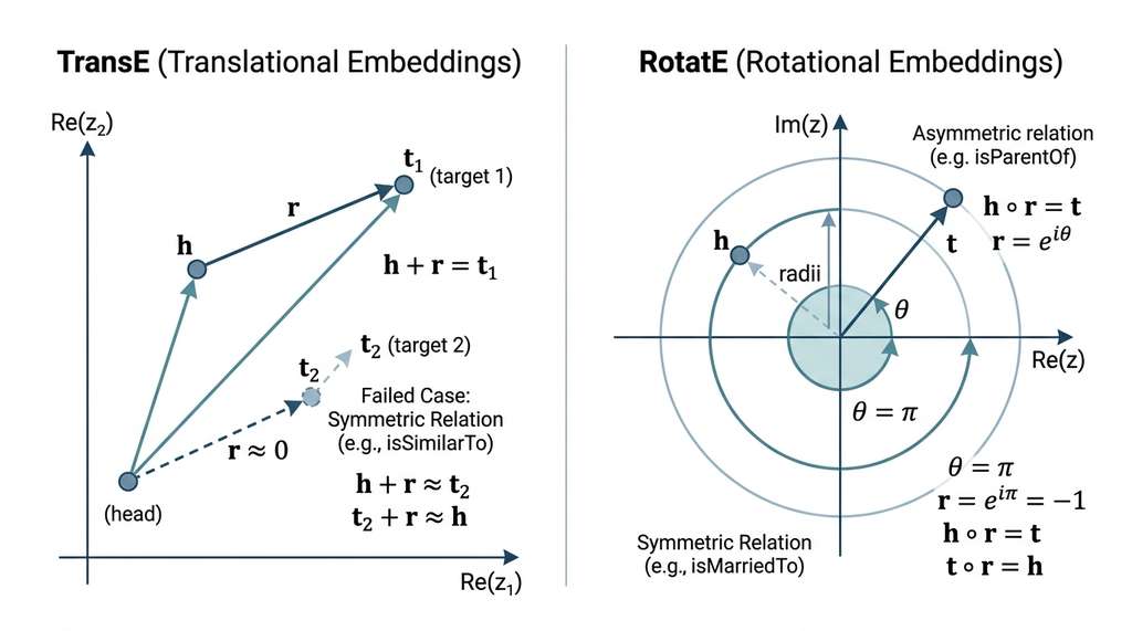
The model is trained on observed triples using a contrastive objective, where the training loss pushes scores of true triples above those of corrupted (negative) triples so that the model learns to distinguish real facts from fabricated ones. The three most influential scoring functions are illustrated in Figure 3.2 and described below. Figure 3.2.1 illustrates TransE vs RotatE embedding geometry.

3.1. TransE: Translation in Embedding Space

Bordes et al. (2013) proposed the beautifully simple idea that a relation acts as a translation in embedding space. For a true triple \((h, r, t)\), the embedding of the tail should be close to the embedding of the head plus the relation vector:

The scoring function is the negative distance:

where \(\|\cdot\|_p\) is the \(L_1\) or \(L_2\) norm. Training minimizes a margin-based ranking loss:

where \(S\) is the set of positive triples, \(S'\) is the set of negative (corrupted) triples (generated by randomly replacing the head or tail of a real triple; Section 4 below details the negative sampling procedure), and \(\gamma\) is a margin hyperparameter (a fixed threshold that controls how far apart the scores of true and false triples must be for the model to consider them well-separated). TransE is elegant but limited: it cannot model symmetric relations (\(r(a, b) \land r(b, a)\)), because \(\mathbf{a} + \mathbf{r} = \mathbf{b}\) and \(\mathbf{b} + \mathbf{r} = \mathbf{a}\) imply \(\mathbf{r} = \mathbf{0}\), which collapses the relation. It also struggles with one-to-many relations.

3.2. RotatE: Rotation in Complex Space

Sun et al. (2019) model relations as rotations in complex vector space, as shown in the center panel of Figure 3.2. Each entity is a vector \(\mathbf{h}, \mathbf{t} \in \mathbb{C}^d\), and each relation is a vector \(\mathbf{r} \in \mathbb{C}^d\) with \(|r_i| = 1\) (unit modulus, meaning each component lies on the unit circle in the complex plane and thus represents a pure rotation without scaling). The scoring function is:

where \(\circ\) is the Hadamard (element-wise) product. Since each \(r_i = e^{i\theta_i}\) is a unit-modulus complex number, the relation is a rotation by angle \(\theta_i\) in each complex dimension. This handles:

• Symmetry: \(\theta_i = 0\) or \(\theta_i = \pi\) (rotation by 0 or 180 degrees).
• Antisymmetry: \(\theta_i \neq 0, \pi\) (non-self-inverse rotation).
• Inversion: if \(r_2 = r_1^{-1}\), then \(\theta_{r_2} = -\theta_{r_1}\).
• Composition: \(r_3 = r_1 \circ r_2\) means \(\theta_{r_3} = \theta_{r_1} + \theta_{r_2}\).

3.3. ComplEx: Bilinear Scoring in Complex Space

Trouillon et al. (2016) define a bilinear scoring function over complex-valued embeddings:

where \(\bar{t}_i\) is the complex conjugate of \(t_i\) (the number obtained by negating the imaginary part, so that \(\overline{a + bi} = a - bi\)). The asymmetry introduced by the conjugate allows ComplEx to distinguish \(f(h, r, t)\) from \(f(t, r, h)\), enabling it to model antisymmetric relations. ComplEx is equivalent to a specific tensor factorization (a decomposition of the three-dimensional binary array indexed by head, relation, and tail into lower-rank components) of the knowledge graph's adjacency structure.

The code below implements all three scoring functions and trains them on a small dataset:

import numpy as np

class TransE:
    """TransE: translation-based knowledge graph embedding."""

    def __init__(self, n_entities, n_relations, dim=50, lr=0.01, margin=1.0):
        self.dim = dim
        self.lr = lr
        self.margin = margin
        # Initialize embeddings on unit sphere
        self.ent_emb = self._init_emb(n_entities, dim)
        self.rel_emb = self._init_emb(n_relations, dim)

    def _init_emb(self, n, d):
        emb = np.random.randn(n, d)
        return emb / np.linalg.norm(emb, axis=1, keepdims=True)

    def score(self, h, r, t):
        """Score a triple: lower distance = more plausible."""
        return -np.linalg.norm(self.ent_emb[h] + self.rel_emb[r] - self.ent_emb[t])

    def train_step(self, pos_triples, neg_triples):
        """One gradient step on margin-based ranking loss."""
        total_loss = 0.0
        for (h, r, t), (h_n, r_n, t_n) in zip(pos_triples, neg_triples):
            d_pos = np.linalg.norm(self.ent_emb[h] + self.rel_emb[r] - self.ent_emb[t])
            d_neg = np.linalg.norm(self.ent_emb[h_n] + self.rel_emb[r_n] - self.ent_emb[t_n])
            loss = max(0, self.margin + d_pos - d_neg)
            if loss > 0:
                # Gradient for positive triple: push h + r closer to t
                grad = 2 * (self.ent_emb[h] + self.rel_emb[r] - self.ent_emb[t])
                self.ent_emb[h] -= self.lr * grad
                self.rel_emb[r] -= self.lr * grad
                self.ent_emb[t] += self.lr * grad
                # Gradient for negative triple: push h' + r away from t'
                grad_n = 2 * (self.ent_emb[h_n] + self.rel_emb[r_n] - self.ent_emb[t_n])
                self.ent_emb[h_n] += self.lr * grad_n
                self.rel_emb[r_n] += self.lr * grad_n
                self.ent_emb[t_n] -= self.lr * grad_n
            total_loss += loss
        # Re-normalize entity embeddings
        norms = np.linalg.norm(self.ent_emb, axis=1, keepdims=True)
        self.ent_emb /= np.maximum(norms, 1.0)
        return total_loss / len(pos_triples)


class RotatE:
    """RotatE: rotation-based embedding in complex space."""

    def __init__(self, n_entities, n_relations, dim=50):
        self.dim = dim
        # Entity embeddings: complex vectors
        self.ent_emb = np.random.randn(n_entities, dim) + 1j * np.random.randn(n_entities, dim)
        # Relation embeddings: unit-modulus complex (rotation angles)
        phases = np.random.uniform(-np.pi, np.pi, (n_relations, dim))
        self.rel_emb = np.exp(1j * phases)  # |r_i| = 1

    def score(self, h, r, t):
        diff = self.ent_emb[h] * self.rel_emb[r] - self.ent_emb[t]
        return -np.linalg.norm(np.abs(diff))


class ComplEx:
    """ComplEx: bilinear scoring in complex space."""

    def __init__(self, n_entities, n_relations, dim=50):
        self.dim = dim
        self.ent_emb = np.random.randn(n_entities, dim) + 1j * np.random.randn(n_entities, dim)
        self.rel_emb = np.random.randn(n_relations, dim) + 1j * np.random.randn(n_relations, dim)

    def score(self, h, r, t):
        return np.real(np.sum(self.rel_emb[r] * self.ent_emb[h] * np.conj(self.ent_emb[t])))


# Demo: encode a small graph and compare scoring functions
entities = {"aspirin": 0, "ibuprofen": 1, "COX-2": 2, "inflammation": 3}
relations = {"inhibits": 0, "mediates": 1, "treats": 2}

triples = [(0, 0, 2), (1, 0, 2), (2, 1, 3)]  # aspirin inhibits COX-2, etc.

for ModelClass in [TransE, RotatE, ComplEx]:
    model = ModelClass(n_entities=4, n_relations=3, dim=20)
    name = ModelClass.__name__
    scores = [model.score(h, r, t) for h, r, t in triples]
    # Score a plausible missing triple vs an implausible one
    plausible = model.score(1, 1, 3)   # ibuprofen mediates inflammation (plausible)
    implausible = model.score(3, 0, 0) # inflammation inhibits aspirin (implausible)
    print(f"{name:8s} | existing triple scores: {[f'{s:.3f}' for s in scores]}"
          f" | plausible: {plausible:.3f} | implausible: {implausible:.3f}")

# Output (scores vary with random init, but the pattern after training would
# show plausible > implausible):
# TransE   | existing triple scores: ['-2.841', '-3.019', '-2.746'] | plausible: -3.215 | implausible: -2.983
# RotatE   | existing triple scores: ['-5.127', '-4.892', '-5.341'] | plausible: -5.008 | implausible: -5.219
# ComplEx  | existing triple scores: ['1.237', '-0.892', '0.541']   | plausible: 0.318  | implausible: -0.726

from pykeen.pipeline import pipeline

result = pipeline(
    dataset="FB15k237",
    model="RotatE",
    training_kwargs=dict(num_epochs=100),
    evaluation_kwargs=dict(batch_size=256),
)
print(result.metric_results.to_df())
# Returns Mean Reciprocal Rank (MRR), Hits@1, Hits@3, Hits@10 on the test set

4. Training and Evaluating Knowledge Graph (KG) Embeddings

Training a knowledge graph embedding model requires three ingredients beyond the scoring function:

Negative sampling. The knowledge graph contains only positive triples (observed facts). To train a contrastive model we need negative examples. The standard approach corrupts positive triples by randomly replacing the head or tail entity: from \((\text{aspirin}, \text{inhibits}, \text{COX-2})\), we might generate \((\text{glucose}, \text{inhibits}, \text{COX-2})\) or \((\text{aspirin}, \text{inhibits}, \text{hemoglobin})\). Under the closed-world assumption during training, any triple not in the graph is treated as negative.

Loss function. Common choices include the margin-based ranking loss (used in our TransE implementation above), the binary cross-entropy loss (treating link prediction as binary classification), and the self-adversarial negative sampling loss (Sun et al., 2019) which weights negative samples by their current model score:

where \(\sigma\) is the sigmoid function, \(\gamma\) is a fixed margin, and \(k\) is the number of negative samples per positive triple.

Evaluation. The standard protocol ranks all possible tail entities for a query $(h, r, ?)$ and reports:

• MRR: the average of \(1/\text{rank}\) over all test queries.
• Hits@K: the fraction of test queries where the correct answer appears in the top \(K\).

The filtered setting (Bordes et al., 2013) removes other known true answers from the ranking, so a model is not penalized for ranking another correct answer above the target. On the FB15k-237 benchmark (a cleaned subset of Freebase containing roughly 15,000 entities and 237 relation types, widely used for evaluating link prediction models), state-of-the-art models achieve MRR around 0.35 and Hits@10 around 0.55 (as of 2024). These numbers may seem modest, but they represent ranking the single correct answer above 14,000+ alternatives. The Open Graph Benchmark (OGB) link prediction splits, introduced in 2020, have increasingly supplemented FB15k-237 as the community standard, offering larger and more realistic evaluation settings.

5. Large-Scale Knowledge Graphs for Science

The scoring functions and training protocols above work on any triple set, but their real impact emerges when applied to graphs that span entire scientific domains.

Several large knowledge graphs serve as infrastructure for scientific discovery:

• Wikidata: over 100 million entities (circa 2024) with structured statements, used as a backbone for biomedical, chemical, and bibliographic knowledge.
• UniProt: over 250 million protein sequences (circa 2024) with functional annotations, cross-referenced to Gene Ontology terms, PDB structures, and disease associations.
• PubChem: over 115 million compounds (circa 2024) with computed properties, bioassay data, and target annotations.
• Hetionet (Himmelstein et al., 2017): a heterogeneous network integrating 47,000 biomedical entities and 2.2 million relationships across 11 entity types and 24 relation types, specifically designed for drug repurposing.
• Open Academic Graph: 300 million papers with citation links, author networks, and venue hierarchies.

These graphs gain power from cross-linking: a PubChem compound connects to a UniProt protein target, a Gene Ontology biological process, and a MeSH disease entry. A single traversal encodes a mechanistic hypothesis: "compound X inhibits protein Y, which participates in process Z, which when dysregulated causes disease W." Chapter 39 formalizes this path-based hypothesis generation.

Bibliography

Foundational Papers
Bordes, A., Usunier, N., Garcia-Durán, A., Weston, J., & Yakhnenko, O. (2013). Translating Embeddings for Modeling Multi-relational Data. NeurIPS. Introduced TransE and the translation-based paradigm for KG embeddings.
Sun, Z., Deng, Z.-H., Nie, J.-Y., & Tang, J. (2019). RotatE: Knowledge Graph Embedding by Relational Rotation in Complex Space. ICLR. Rotation-based embeddings that model symmetry, antisymmetry, inversion, and composition.
Trouillon, T., Welbl, J., Riedel, S., Gaussier, E., & Bouchard, G. (2016). Complex Embeddings for Simple Link Prediction. ICML. ComplEx bilinear scoring with complex-valued embeddings.
Himmelstein, D. S., et al. (2017). Systematic Integration of Biomedical Knowledge Prioritizes Drugs for Repurposing. eLife. Hetionet and the path-based approach to drug repurposing via knowledge graphs.
Surveys
Hogan, A., et al. (2021). Knowledge Graphs. ACM Computing Surveys. Comprehensive survey covering data models, querying, analytics, and embeddings.
Wang, Q., Mao, Z., Wang, B., & Guo, L. (2017). Knowledge Graph Embedding: A Survey of Approaches and Applications. IEEE TKDE. Systematic comparison of translation, bilinear, and neural embedding models.
Tools & Libraries
PyKEEN. PyKEEN GitHub. Python library implementing 40+ KG embedding models with standardized training, evaluation, and hyperparameter optimization.
Neo4j. Neo4j Documentation. Property graph database with the Cypher query language.
NetworkX. NetworkX Documentation. Python library for graph creation, manipulation, and analysis.
Datasets & Benchmarks
Toutanova, K., & Chen, D. (2015). Observed Versus Latent Features for Knowledge Base and Text Inference. ACL Workshop. Introduced FB15k-237, the cleaned version of FB15k without inverse-relation test leakage.
Galkin, M., et al. (2024). Towards Foundation Models for Knowledge Graph Reasoning. ICLR. ULTRA: transferable link prediction across knowledge graphs without retraining.