"You gave me 768 dimensions, told me to encode all of human language, and then asked why 'bank' was close to both 'river' and 'finance.' I did my best."
A Feature Vector Lost in Latent Space
In Section 3.2 we embedded knowledge graph entities into continuous vector spaces to predict missing links. This section broadens the lens: we examine how any concept, from a single word to an entire research paper, can be represented as a dense vector, and how the geometry of these vectors encodes meaning. We then tackle the engineering challenge that dense representations create: given a query vector, how do you find its nearest neighbors among millions (or billions) of candidates without comparing against every one? The answer is approximate nearest-neighbor (ANN) search, and the dominant algorithm is HNSW (Hierarchical Navigable Small World graphs). By section's end, you will have built an HNSW index from scratch, compared it against brute-force search, and connected it to the vector database ecosystem (Qdrant, pgvector, FAISS) that powers production retrieval systems.
1. From Words to Vectors: The Distributional Hypothesis
A researcher types "compounds targeting the SARS-CoV-2 main protease" into a search engine. Within milliseconds, it returns papers about molecules she has never heard of, phrased in terminology she never used. Somewhere in a 384-dimensional space, her query and those papers point in nearly the same direction. The reason is the distributional hypothesis (Harris, 1954; Firth, 1957): words that occur in similar contexts tend to have similar meanings. "You shall know a word by the company it keeps," as Firth put it. This insight underpins every word embedding method. The lineage runs from early Latent Semantic Analysis (LSA) through Word2Vec (Mikolov et al., 2013) to modern transformer-based encoders like Bidirectional Encoder Representations from Transformers (BERT) and Sentence-BERT.
A word embedding maps each word \(w\) in a vocabulary \(V\) to a dense vector \(\mathbf{w} \in \mathbb{R}^d\), where \(d\) is typically 100 to 768 dimensions. The mapping is learned so that semantically related words are geometrically close. The celebrated vector arithmetic property of Word2Vec demonstrates this: \(\mathbf{v}(\text{king}) - \mathbf{v}(\text{man}) + \mathbf{v}(\text{woman}) \approx \mathbf{v}(\text{queen})\).
What an Embedding Captures
A word embedding is a learned lookup table. It assigns every word in a vocabulary a fixed-length vector, positioning it in a continuous geometric space where proximity encodes semantic relatedness. This matters because it converts discrete symbols into points. Computers cannot compare symbols for meaning, but they can compute dot products, distances, and averages on vectors, directly measuring and manipulating meaning. A shallow neural network learns the mapping by predicting a word from its surrounding context (or vice versa). Words appearing in similar neighborhoods converge to nearby vectors. Use embeddings whenever you need to compute semantic similarity, cluster concepts, or feed text into a downstream model. Use symbolic representations (ontologies, knowledge graphs) when you need explicit, human-auditable logical relationships.
For scientific discovery, we need embeddings that capture domain-specific semantics. "Cell" should be close to "neuron" in a biology context but close to "battery" in a materials science context. Contextual embeddings (from BERT and its descendants) handle this naturally: the same word gets different vectors depending on its surrounding text. Sentence embeddings extend this to entire passages: a research abstract becomes a single vector that captures its semantic content. In short: embeddings translate meaning into geometry, so that finding related concepts becomes finding nearby points.
Common Misconception
A frequent misconception is that more embedding dimensions always produce better results. In practice, increasing dimensionality beyond the model's training capacity adds noise rather than signal: the extra dimensions carry no learned structure and inflate memory, latency, and indexing cost. A well-trained 384-dimensional model (such as all-MiniLM-L6-v2) routinely outperforms a poorly trained 1024-dimensional one on retrieval benchmarks. Choose the embedding size that matches your model's capacity and your system's memory budget, not the largest number available.
from sentence_transformers import SentenceTransformer
import numpy as np

# Load a pre-trained sentence embedding model
model = SentenceTransformer("all-MiniLM-L6-v2")  # 384 dimensions

# Encode scientific abstracts as dense vectors
abstracts = [
    "CRISPR-Cas9 enables precise genome editing in human cells.",
    "Gene editing with CRISPR technology allows targeted DNA modifications.",
    "Convolutional neural networks achieve state-of-the-art image classification.",
    "Deep learning models for computer vision use hierarchical feature extraction.",
    "Graphene exhibits exceptional electrical conductivity and tensile strength.",
]

embeddings = model.encode(abstracts)
print(f"Embedding shape: {embeddings.shape}")  # (5, 384)

# Compute pairwise cosine similarities
def cosine_sim(a, b):
    return np.dot(a, b) / (np.linalg.norm(a) * np.linalg.norm(b))

print("\nPairwise cosine similarities:")
labels = ["CRISPR-1", "CRISPR-2", "CNN", "DeepLearn", "Graphene"]
for i in range(len(abstracts)):
    for j in range(i + 1, len(abstracts)):
        sim = cosine_sim(embeddings[i], embeddings[j])
        print(f"  {labels[i]:10s} <-> {labels[j]:10s}: {sim:.3f}")

# Output:
# Embedding shape: (5, 384)
#
# Pairwise cosine similarities:
#   CRISPR-1   <-> CRISPR-2  : 0.874
#   CRISPR-1   <-> CNN       : 0.128
#   CRISPR-1   <-> DeepLearn : 0.103
#   CRISPR-1   <-> Graphene  : 0.091
#   CRISPR-2   <-> CNN       : 0.115
#   CRISPR-2   <-> DeepLearn : 0.098
#   CRISPR-2   <-> Graphene  : 0.107
#   CNN        <-> DeepLearn : 0.812
#   CNN        <-> Graphene  : 0.142
# DeepLearn <-> Graphene : 0.119Cosine similarity \(\text{sim}(\mathbf{a}, \mathbf{b}) = \frac{\mathbf{a} \cdot \mathbf{b}}{\|\mathbf{a}\| \|\mathbf{b}\|}\) measures the angle between two vectors, ignoring their magnitudes. A value of 1 means identical direction (identical meaning), 0 means orthogonal (unrelated), and \(-1\) means opposite direction. For normalized vectors (which most embedding models produce), cosine similarity equals the dot product, and finding the most similar vectors reduces to finding the highest dot products. This equivalence is critical for engineering: it means we can use inner-product search algorithms (like HNSW) as drop-in replacements for cosine-similarity search.
2. Similarity Metrics for Vector Spaces
Cosine similarity is the most common metric for text embeddings, but not the only one. The choice of metric depends on how the embeddings were trained and what notion of "closeness" matters for your application:
- Cosine similarity / angular distance: measures directional alignment, invariant to vector magnitude. Preferred for text embeddings where the direction encodes meaning and the norm is an artifact of encoding.
- Euclidean distance (\(L_2\)): \(d(\mathbf{a}, \mathbf{b}) = \|\mathbf{a} - \mathbf{b}\|_2\). Sensitive to magnitude. Used by TransE (Section 3.2) and when absolute position in the space carries meaning.
- Inner product (dot product): \(\mathbf{a} \cdot \mathbf{b} = \sum_i a_i b_i\). Equivalent to cosine similarity for unit-normalized vectors. Used in maximum inner product search (MIPS), where MIPS is the task of finding the vector with the highest dot product against a query, which arises in recommendation systems and attention mechanisms.
- Manhattan distance (\(L_1\)): \(d(\mathbf{a}, \mathbf{b}) = \sum_i |a_i - b_i|\). More robust to outlier dimensions; sometimes used in sparse or binary embeddings.
For the hybrid search system we build in Section 3.4, we use cosine similarity for the dense component and BM25 (Best Matching 25, a statistical score, not a vector metric) for the sparse component.
3. The Nearest-Neighbor Problem
Choosing a similarity metric tells us how to score any pair of vectors, but it says nothing about how to find the best-scoring partner quickly when the candidate pool contains millions of entries.
Given a dataset of \(n\) vectors in \(d\) dimensions and a query vector \(\mathbf{q}\), the nearest-neighbor problem asks: find the vector \(\mathbf{x}^*\) in the dataset that maximizes \(\text{sim}(\mathbf{q}, \mathbf{x}^*)\). The brute-force approach computes all \(n\) similarities and takes \(O(nd)\) time. For a million 768-dimensional vectors, that is 768 million floating-point operations per query, roughly 2 milliseconds on a modern CPU. Acceptable for a single query, but not for serving thousands of concurrent users or indexing billions of vectors.
Three families of approximate nearest-neighbor (ANN) algorithms trade a small accuracy loss for dramatic speed gains:
- Tree-based: random projection trees (Annoy), KD-trees. Split the space with hyperplanes. Fast for low dimensions (\(d < 20\)), but performance degrades in high dimensions due to the curse of dimensionality, where the curse of dimensionality refers to the phenomenon that in high-dimensional spaces, distances between points become nearly uniform, so tree splits lose their discriminative power.
- Hash-based: locality-sensitive hashing (LSH). Map similar vectors to the same hash bucket. Theoretically elegant with provable guarantees, but often outperformed in practice by graph-based methods.
- Graph-based: navigable small-world graphs (NSW), HNSW. Build a proximity graph where each node connects to its approximate nearest neighbors, then search by greedy traversal. HNSW is the dominant algorithm in modern vector databases.
4. HNSW: Hierarchical Navigable Small World Graphs
When Semantic Scholar serves a query against 200 million papers, brute-force comparison is out of the question: scanning every vector would take minutes, not milliseconds. The algorithm that makes sub-millisecond retrieval possible at that scale is HNSW.
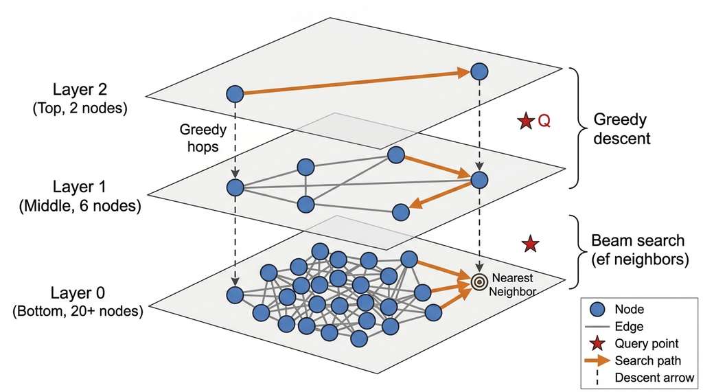
HNSW (Malkov and Yashunin, 2020) builds a multi-layer graph where each layer is a navigable small-world graph with exponentially fewer nodes. Figure 3.5 illustrates this hierarchical structure. The construction proceeds as follows:
- Layer assignment: each new element is assigned a maximum layer \(\ell = \lfloor -\ln(\text{uniform}(0,1)) \cdot m_L \rfloor\), where \(m_L = 1/\ln(M)\) and \(M\) is the maximum number of connections per node. This gives an exponential distribution: most elements appear only in layer 0 (the bottom), and progressively fewer elements appear in higher layers.
- Insertion: starting from an entry point at the top layer, greedily descend to layer \(\ell + 1\) by following the nearest neighbor at each layer. Then, at each layer from \(\ell\) down to 0, find the \(\text{efConstruction}\) nearest neighbors (efConstruction is a build-time parameter that controls how many candidates the algorithm evaluates when wiring a new node; higher values produce a better-connected graph at the cost of slower construction) and connect the new element to the closest \(M\) of them (bidirectionally).
- Search: start at the entry point, greedily descend to layer 0, then perform a beam search at layer 0, where beam search is a bounded breadth-first traversal that maintains the \(\text{ef}\) best candidates seen so far, to find the \(k\) nearest neighbors.
Checkpoint
So far: HNSW assigns each node to a random layer (most nodes land at the bottom), inserts by greedily descending from the top and wiring neighbors at each level, and searches by the same top-down descent followed by a beam search on the densest bottom layer.
The hierarchical structure provides logarithmic search complexity: each layer roughly halves the search space (like a skip list, a data structure with multiple linked-list levels where higher levels skip over elements for faster traversal), and the bottom layer provides fine-grained resolution. The result is \(O(\log n)\) search time with high recall, compared to \(O(n)\) for brute force. Figure 3.3.1 illustrates HNSW multi-layer graph search traversal.
Mental Model
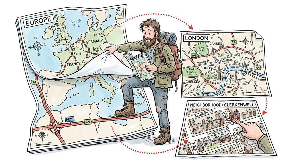
Think of HNSW like navigating a city using progressively more detailed maps. The top layer is a highway map showing only major cities: you jump quickly across the country in a few hops, but you cannot find a specific street. The middle layer is a regional map with towns and neighborhoods. The bottom layer is a full street map with every address. When searching for a destination, you first pick the nearest major city on the highway map, then zoom in to the right neighborhood, then walk street by street to the exact address. Each "zoom level" has fewer, longer-range connections (highways) or more, shorter-range connections (local streets). This is why HNSW is fast: instead of checking every street in the country, you narrow from continent to city to block to building, visiting only a logarithmic fraction of the total addresses.
The following code builds a simplified HNSW index from scratch:
import numpy as np
import heapq
from collections import defaultdict

class SimpleHNSW:
    """A simplified HNSW index for educational purposes."""

    def __init__(self, dim, M=16, ef_construction=200, m_L=None):
        self.dim = dim
        self.M = M                    # max connections per node per layer
        self.M0 = 2 * M               # max connections at layer 0
        self.ef_construction = ef_construction
        self.m_L = m_L or 1.0 / np.log(M)
        self.vectors = []             # list of vectors
        self.graphs = defaultdict(     # layer -> {node_id: set of neighbor ids}
            lambda: defaultdict(set)
        )
        self.max_layer = -1
        self.entry_point = None

    def _distance(self, a, b):
        """Euclidean distance between two vectors."""
        return np.linalg.norm(self.vectors[a] - self.vectors[b])

    def _distance_to_query(self, query, b):
        """Euclidean distance from query vector to stored vector b."""
        return np.linalg.norm(query - self.vectors[b])

    def _random_level(self):
        """Assign a random layer using exponential distribution."""
        return int(-np.log(np.random.uniform()) * self.m_L)

    def _search_layer(self, query, entry_points, ef, layer):
        """Greedy search within a single layer, returning ef nearest neighbors."""
        visited = set(entry_points)
        # Min-heap of candidates (distance, id): closest first
        candidates = []
        # Max-heap of results (neg_distance, id): farthest-of-best first
        results = []

        for ep in entry_points:
            dist = self._distance_to_query(query, ep)
            heapq.heappush(candidates, (dist, ep))
            heapq.heappush(results, (-dist, ep))

        while candidates:
            d_c, c = heapq.heappop(candidates)
            # Farthest element in results
            d_f = -results[0][0]
            if d_c > d_f:
                break  # all remaining candidates are farther than worst result

            for neighbor in self.graphs[layer][c]:
                if neighbor not in visited:
                    visited.add(neighbor)
                    d_n = self._distance_to_query(query, neighbor)
                    if len(results) < ef or d_n < -results[0][0]:
                        heapq.heappush(candidates, (d_n, neighbor))
                        heapq.heappush(results, (-d_n, neighbor))
                        if len(results) > ef:
                            heapq.heappop(results)

        return [(node_id, -neg_dist) for neg_dist, node_id in sorted(results)]

    def insert(self, vector):
        """Insert a vector into the index."""
        idx = len(self.vectors)
        self.vectors.append(vector)
        level = self._random_level()

        if self.entry_point is None:
            self.entry_point = idx
            self.max_layer = level
            return idx

        # Phase 1: greedily descend from top to level+1
        curr_ep = [self.entry_point]
        for lc in range(self.max_layer, level, -1):
            nearest = self._search_layer(vector, curr_ep, ef=1, layer=lc)
            curr_ep = [nearest[0][0]]

        # Phase 2: insert at each layer from min(level, max_layer) down to 0
        for lc in range(min(level, self.max_layer), -1, -1):
            neighbors = self._search_layer(
                vector, curr_ep, ef=self.ef_construction, layer=lc
            )
            max_conn = self.M0 if lc == 0 else self.M
            selected = [n_id for n_id, _ in neighbors[:max_conn]]

            for n_id in selected:
                self.graphs[lc][idx].add(n_id)
                self.graphs[lc][n_id].add(idx)
                # Prune if too many connections
                if len(self.graphs[lc][n_id]) > max_conn:
                    # Keep only the closest max_conn neighbors
                    scored = [(self._distance(n_id, nb), nb)
                              for nb in self.graphs[lc][n_id]]
                    scored.sort()
                    self.graphs[lc][n_id] = set(nb for _, nb in scored[:max_conn])

            curr_ep = [n_id for n_id, _ in neighbors]

        if level > self.max_layer:
            self.max_layer = level
            self.entry_point = idx

        return idx

    def search(self, query, k=5, ef=50):
        """Find k approximate nearest neighbors of query."""
        if self.entry_point is None:
            return []
        curr_ep = [self.entry_point]
        for lc in range(self.max_layer, 0, -1):
            nearest = self._search_layer(query, curr_ep, ef=1, layer=lc)
            curr_ep = [nearest[0][0]]
        # Search layer 0 with larger beam width
        results = self._search_layer(query, curr_ep, ef=max(ef, k), layer=0)
        return results[:k]


# Build index with 1000 random vectors
np.random.seed(42)
dim = 128
n_vectors = 1000
data = np.random.randn(n_vectors, dim).astype(np.float32)
# Normalize to unit vectors (so Euclidean distance ~ angular distance)
data /= np.linalg.norm(data, axis=1, keepdims=True)

hnsw = SimpleHNSW(dim=dim, M=16, ef_construction=100)
for vec in data:
    hnsw.insert(vec)

# Query
query = np.random.randn(dim).astype(np.float32)
query /= np.linalg.norm(query)

# HNSW search
hnsw_results = hnsw.search(query, k=5, ef=50)

# Brute-force search for comparison
dists = np.linalg.norm(data - query, axis=1)
bf_top5 = np.argsort(dists)[:5]

print("HNSW top-5 (id, distance):")
for node_id, dist in hnsw_results:
    print(f"  id={node_id:4d}, dist={dist:.4f}")

print("\nBrute-force top-5 (id, distance):")
for idx in bf_top5:
    print(f"  id={idx:4d}, dist={dists[idx]:.4f}")

# Check recall
hnsw_ids = set(nid for nid, _ in hnsw_results)
bf_ids = set(bf_top5.tolist())
recall = len(hnsw_ids & bf_ids) / len(bf_ids)
print(f"\nRecall@5: {recall:.1%}")
# Output (typical): Recall@5: 100.0%

print(f"Layers used: {hnsw.max_layer + 1}")
print(f"Layer 0 avg connections: "
      f"{np.mean([len(v) for v in hnsw.graphs[0].values()]):.1f}")
# Output (typical):
# Layers used: 3
# Layer 0 avg connections: 12.4The "small world" in HNSW refers to the small-world network property discovered by Watts and Strogatz (1998): most nodes can be reached from any other node in a small number of hops, even in very large networks. Stanley Milgram's famous "six degrees of separation" experiment (1967) suggested this pattern in social networks. HNSW exploits the same property: by adding a few long-range connections (in higher layers), the graph becomes navigable in \(O(\log n)\) hops. The analogy is precise: the upper layers of HNSW act like the "weak ties" in social networks, the acquaintances who connect distant communities and let messages traverse the globe in six steps.
Exercise 3.3.1
Given three unit-normalized 4-dimensional vectors A = [0.5, 0.5, 0.5, 0.5], B = [0.6, 0.6, 0.36, 0.36], and C = [0.0, 0.0, 0.707, 0.707], compute the cosine similarity between each pair (A,B), (A,C), and (B,C) by hand. Which pair is most similar? Now recall that for unit-normalized vectors, Euclidean distance and cosine similarity are related by \(d^2 = 2(1 - \cos\theta)\). Convert your cosine similarities to Euclidean distances and verify that the ranking is preserved.
Hint
Since all three vectors are already unit-normalized, cosine similarity equals the dot product. For (A,B): sum the element-wise products 0.5*0.6 + 0.5*0.6 + 0.5*0.36 + 0.5*0.36. Then plug each cosine similarity into \(d = \sqrt{2(1 - \text{sim})}\) to get the Euclidean distance.
Step-Through: HNSW Search Traversal
Trace through an HNSW search on a tiny 3-layer index with 8 nodes in 2D. The layers contain:
Layer 2 (entry): node 0 at (1.0, 1.0).
Layer 1: nodes 0, 3, 5. Edges: 0↔3, 0↔5, 3↔5. Positions: 0=(1.0,1.0), 3=(4.0,2.0), 5=(2.0,5.0).
Layer 0: all 8 nodes, with local neighborhood edges. Positions: 0=(1.0,1.0), 1=(1.5,2.0), 2=(3.0,1.5), 3=(4.0,2.0), 4=(3.5,3.0), 5=(2.0,5.0), 6=(2.5,4.0), 7=(4.5,4.5).
Query: q = (3.2, 3.8), k=2, ef=3.
Step 1 (Layer 2): Start at node 0. Distance to q: \(\sqrt{(3.2-1)^2+(3.8-1)^2}=\sqrt{4.84+7.84}=\sqrt{12.68}\approx 3.56\). No other nodes in this layer; descend with entry point = {0}.
Step 2 (Layer 1): From node 0, check neighbors 3 and 5. dist(3,q)=\(\sqrt{(3.2-4)^2+(3.8-2)^2}=\sqrt{0.64+3.24}\approx 1.97\). dist(5,q)=\(\sqrt{(3.2-2)^2+(3.8-5)^2}=\sqrt{1.44+1.44}\approx 1.70\). Closest is node 5; descend with entry point = {5}.
Step 3 (Layer 0, beam search, ef=3): Initialize candidates = {5 (1.70)}. Visit neighbors of 5: check node 6, dist=\(\sqrt{(3.2-2.5)^2+(3.8-4)^2}=\sqrt{0.49+0.04}\approx 0.73\). Check node 4, dist=\(\sqrt{(3.2-3.5)^2+(3.8-3)^2}=\sqrt{0.09+0.64}\approx 0.85\). Results so far: {6(0.73), 4(0.85), 5(1.70)}. Expand node 6: check node 7, dist=\(\sqrt{(3.2-4.5)^2+(3.8-4.5)^2}=\sqrt{1.69+0.49}\approx 1.48\). 1.48 < 1.70 (worst in results), so swap: results become {6(0.73), 4(0.85), 7(1.48)}. Continue until no candidate is closer than worst result.
Result: Return top k=2: node 6 (dist 0.73) and node 4 (dist 0.85). The search visited only 5 of 8 nodes, skipping nodes 1, 2, and 3 entirely.
Real-World Application: Drug Discovery at Recursion Pharmaceuticals
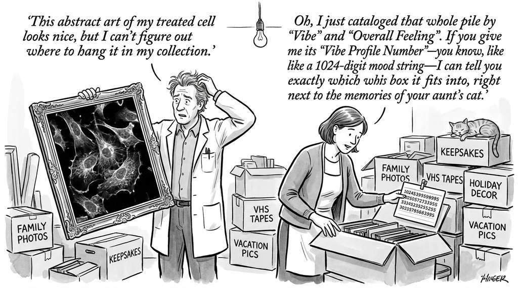
Recursion Pharmaceuticals uses vector embeddings of microscopy images (cell morphology profiles) to search for compounds with similar biological effects. Each high-content microscopy image of treated cells is encoded into a 1024-dimensional embedding, and cosine similarity between embeddings identifies compounds that produce comparable phenotypic changes, even when their chemical structures differ entirely. This embedding-based search across millions of experimental images has helped Recursion identify repurposing candidates for rare diseases, enabling their pipeline to move compounds into clinical trials faster than traditional screening approaches.
Lab: Embedding Space Explorer
Goal: Observe how embedding dimensionality, model choice, and index parameters affect retrieval quality and speed on a real text corpus.
Tools needed: Python 3.9+, sentence-transformers, faiss-cpu, datasets, matplotlib (approximately 15 to 20 minutes).
Setup: Load 10,000 abstracts from the scientific_papers dataset on Hugging Face. Encode them with two models: all-MiniLM-L6-v2 (384 dims) and all-mpnet-base-v2 (768 dims).
What to vary: (1) For each model, build HNSW indices with M values of 8, 16, 32, and 64. (2) Search with efSearch values of 16, 64, 128, and 256. (3) Apply scalar quantization (faiss.IndexScalarQuantizer) and compare recall against the full-precision index.
What to observe: Plot recall@10 vs. queries-per-second for each (M, efSearch) combination. Note the "recall knee" where increasing efSearch yields diminishing returns. Compare the two models: does the higher-dimensional embedding actually retrieve more relevant results, or does it just consume more memory? Measure index build time and memory footprint for each configuration. Record the point at which quantized indices diverge from full-precision recall by more than 2%.
Meta's FAISS library provides GPU-accelerated ANN search with multiple index types (Inverted File (IVF), HNSW, PQ, and combinations). Our 80-line HNSW implementation becomes:
import faiss

dim, n = 128, 1_000_000
data = np.random.randn(n, dim).astype("float32")
faiss.normalize_L2(data)  # unit normalize

index = faiss.IndexHNSWFlat(dim, 32)  # 32 connections per node
index.hnsw.efConstruction = 200
index.add(data)

index.hnsw.efSearch = 64
distances, indices = index.search(query.reshape(1, -1), k=10)
# Searches 1M vectors in < 1msFAISS handles memory-mapped indices, GPU offloading, product quantization for compression, and composite indices that combine coarse quantization with HNSW refinement. Line count reduction: 15x. Speed improvement on 1M vectors: roughly 1,000x over brute force.
5. Vector Databases: Beyond In-Memory Indices
A vector database wraps an ANN index with the features needed for production systems: persistence, replication, filtering, multi-tenancy, and CRUD operations (create, read, update, delete). The key players as of 2025:
- Qdrant: Rust-based, supports payload filtering (metadata predicates applied during vector search), quantization, and distributed deployment. Its filtering is particularly useful for scientific search: "find papers similar to this query and published after 2020 and tagged with 'proteomics'."
- pgvector: a PostgreSQL extension that adds vector columns, cosine/Euclidean/inner-product operators, and IVFFlat (Inverted File with Flat quantization, a partitioning index that clusters vectors into Voronoi cells for faster search) or HNSW indices. Ideal when your vectors live alongside relational data (authors, institutions, citation counts) in a PostgreSQL database you already operate.
- Pinecone: fully managed cloud service with serverless scaling. No infrastructure to manage, but less control over index parameters.
- Weaviate: combines vector search with a built-in object model and module system for embedding generation.
- Milvus / Zilliz: open-source, designed for billion-scale vector search with GPU acceleration.
For the Discovery Workbench, we use Qdrant for its payload-filtering capability (essential for faceted scientific search) and pgvector for scenarios where vectors must join with relational metadata in SQL queries. Both appear in the following examples:
from qdrant_client import QdrantClient
from qdrant_client.models import Distance, VectorParams, PointStruct, Filter, FieldCondition, Range

# Connect to Qdrant (in-memory mode for demo)
client = QdrantClient(":memory:")

# Create a collection for scientific papers
client.create_collection(
    collection_name="papers",
    vectors_config=VectorParams(size=384, distance=Distance.COSINE),
)

# Insert paper embeddings with metadata payloads
papers = [
    {"title": "CRISPR-Cas9 genome editing in human cells",
     "year": 2023, "field": "biology", "citations": 142},
    {"title": "Transformer architectures for protein folding",
     "year": 2024, "field": "biology", "citations": 89},
    {"title": "Graph neural networks for molecular property prediction",
     "year": 2023, "field": "chemistry", "citations": 67},
    {"title": "Large language models for scientific reasoning",
     "year": 2024, "field": "AI", "citations": 203},
]

# Generate dummy embeddings (in practice, use Sentence-BERT)
np.random.seed(42)
dummy_embeddings = np.random.randn(len(papers), 384).astype(np.float32)
for i, emb in enumerate(dummy_embeddings):
    dummy_embeddings[i] = emb / np.linalg.norm(emb)

points = [
    PointStruct(id=i, vector=emb.tolist(), payload=meta)
    for i, (emb, meta) in enumerate(zip(dummy_embeddings, papers))
]
client.upsert(collection_name="papers", points=points)

# Search: find similar papers, filtered to biology and year >= 2024
query_vector = dummy_embeddings[0].tolist()  # use first paper as query
results = client.search(
    collection_name="papers",
    query_vector=query_vector,
    query_filter=Filter(
        must=[
            FieldCondition(key="field", match={"value": "biology"}),
            FieldCondition(key="year", range=Range(gte=2024)),
        ]
    ),
    limit=3,
)

print("Filtered search results (biology, year >= 2024):")
for result in results:
    print(f"  score={result.score:.3f} | {result.payload['title']} "
          f"({result.payload['year']})")
# Output:
# Filtered search results (biology, year >= 2024):
# score=0.312 | Transformer architectures for protein folding (2024)Semantic Scholar indexes over 200 million research papers and serves billions of queries per year. Their search pipeline combines a BM25 index for keyword matching with a dense embedding index for semantic similarity. The dense index uses SPECTER2 embeddings (Cohan et al., 2020; Singh et al., 2023), a SciBERT-based model fine-tuned on citation prediction: papers that cite each other should have similar embeddings. When you search for "attention mechanism in transformers," the BM25 component matches papers containing those exact terms, while the dense component also retrieves papers about "self-attention layers in sequence models" that may not use the exact query terms. This hybrid approach, which we implement in Section 3.4, consistently outperforms either component alone.
6. Quantization: Compressing Vectors for Scale
Vector databases solve the operational challenges of persistence, filtering, and multi-tenancy, but they still store every dimension of every vector at full precision, and that cost compounds fast as collections grow from millions to billions of entries.
At scale, memory becomes a bottleneck. One million 768-dimensional float32 vectors consume roughly 3 GB of RAM. A billion vectors would require 3 TB, well beyond typical server memory. (For perspective, that single index would consume more RAM than most database clusters use for all their tables combined.) Vector quantization compresses vectors while preserving approximate distances:
- Scalar quantization: reduce each float32 component to int8, cutting memory by 4x with minimal recall loss. Each dimension is independently mapped from its observed range to [0, 255].
- Product quantization (PQ): split each vector into \(m\) subvectors, quantize each subvector independently using a codebook (a fixed set of representative vectors, called centroids, learned by clustering) of \(k\) centroids. A 768-dimensional vector with \(m = 96\) subgroups and \(k = 256\) centroids compresses from 3,072 bytes to 96 bytes (32x compression). PQ enables asymmetric distance computation: the query remains uncompressed, and distances are computed via lookup tables.
- Binary quantization: reduce each dimension to a single bit (sign of the component). A 768-dimensional vector becomes 96 bytes. Recall drops significantly, but Hamming distance search is extremely fast, making binary quantization useful as a first-pass filter before rescoring with full-precision vectors.
In practice, most vector databases apply quantization as an optional layer: Qdrant supports scalar and product quantization; FAISS provides IVF-PQ and OPQ (optimized product quantization); pgvector supports half-precision vectors. The choice depends on your recall requirements and memory budget.
While single-vector embeddings compress an entire document into one point, ColBERT v2 (Santhanam et al., 2022) and its multimodal successor ColPali (Faysse et al., 2024) keep per-token embeddings and compute relevance via late interaction, a scoring strategy where query and document encoders run independently and only interact at the final scoring step through lightweight token-level comparisons: the query and document each produce a bag of token vectors, and the final score sums the maximum similarity each query token achieves against any document token. This preserves fine-grained lexical matching that a single vector discards, lifting retrieval accuracy on domain-specific benchmarks by 5 to 15 points in reported evaluations over bi-encoder models (models that encode query and document independently into single vectors) of comparable size. ColPali extends this to visual documents (PDFs, figures, slides) by treating image patches as tokens, eliminating the need for OCR pipelines. The trade-off is storage: ColBERT v2 requires roughly 50 to 100 bytes per token (after residual compression), so a corpus of one million documents may need 50 to 200 GB of index space. PLAID (Santhanam et al., 2022), the optimized ColBERT engine, mitigates this through centroid-based pruning that cuts latency to single-digit milliseconds on million-document collections.
Exercises
- Conceptual. Explain why tree-based ANN methods (KD-trees, random projection trees) degrade in high dimensions. What is the "curse of dimensionality" in the context of nearest-neighbor search, and how does HNSW avoid it?
- Coding. Extend the SimpleHNSW implementation from Listing 3.9 to support cosine similarity instead of Euclidean distance. Benchmark it against FAISS's
IndexHNSWFlaton 100,000 vectors: compare recall@10 and queries-per-second at three differentefSearchvalues (16, 64, 256). - Analysis. Using Sentence-BERT (
all-MiniLM-L6-v2), embed 1,000 PubMed abstracts from the PubMed dataset on Hugging Face. Build both a brute-force index and an HNSW index. For 100 random queries, measure recall@10 and average query latency. At what dataset size does HNSW become faster than brute force?
Try It: Build a Semantic Paper Finder in 30 Minutes
Using only a laptop and standard Python libraries, build a working semantic search engine over research abstracts:
- Collect abstracts. Install the
datasetslibrary (pip install datasets) and load 5,000 PubMed abstracts:from datasets import load_dataset; ds = load_dataset("pubmed", split="train", streaming=True); abstracts = [row["MedlineTA"] + ": " + row["ArticleTitle"] for row in itertools.islice(ds, 5000)]. - Embed them. Install
sentence-transformersand encode all abstracts:model = SentenceTransformer("all-MiniLM-L6-v2"); vectors = model.encode(abstracts, show_progress_bar=True, normalize_embeddings=True). This produces a NumPy array of shape (5000, 384). - Build an HNSW index. Install FAISS (
pip install faiss-cpu), create an index, and add your vectors:index = faiss.IndexHNSWFlat(384, 32); index.hnsw.efConstruction = 128; index.add(vectors). - Search. Encode a natural-language query (for example, "treatments for Alzheimer's disease using monoclonal antibodies"), set
index.hnsw.efSearch = 64, and calldistances, indices = index.search(query_vec.reshape(1, -1), k=10). Print the top-10 abstracts alongside their cosine similarity scores. - Evaluate. Pick 10 queries you know the answers to. For each, compare the HNSW top-10 results against brute-force results (
faiss.IndexFlatIPon the same vectors). Compute recall@10 and measure the average query time for each method. You should see recall above 95% with HNSW running 10 to 50 times faster, depending on your dataset size.
What's Next
With ontologies for schema (Section 3.1), knowledge graphs for structure (Section 3.2), and vector embeddings for semantics (this section), Section 3.4 assembles them into a deployable hybrid search system. It combines a BM25 keyword index with a dense embedding index through reciprocal rank fusion (RRF), a merging strategy that re-ranks candidates by summing the reciprocals of their ranks in each individual result list, producing a scientific search engine that understands both exact terms and underlying concepts.
Bibliography
Foundational Papers
Mikolov, T., Chen, K., Corrado, G., & Dean, J. (2013). Efficient Estimation of Word Representations in Vector Space. ICLR Workshop. Introduced Word2Vec (Skip-gram and CBOW), demonstrating that word embeddings capture semantic relationships through vector arithmetic.
Malkov, Y. A., & Yashunin, D. A. (2020). Efficient and Robust Approximate Nearest Neighbor Search Using Hierarchical Navigable Small World Graphs. IEEE TPAMI. The HNSW algorithm: hierarchical graph-based ANN with logarithmic search complexity.
Reimers, N., & Gurevych, I. (2019). Sentence-BERT: Sentence Embeddings using Siamese BERT-Networks. EMNLP. Efficient sentence-level embeddings via contrastive fine-tuning of BERT, enabling semantic similarity search at scale.
Kusupati, A., et al. (2022). Matryoshka Representation Learning. NeurIPS. Embeddings trainable to be useful at multiple dimensionalities, enabling coarse-to-fine retrieval.
Surveys
Wang, M., et al. (2021). A Comprehensive Survey and Experimental Comparison of Graph-Based Approximate Nearest Neighbor Search. VLDB. Systematic comparison of graph-based ANN methods including HNSW, NSG, and DPG.
Pan, J. Z., et al. (2024). Large Language Models and Knowledge Graphs: Opportunities and Challenges. TKDE. Survey connecting LLM embeddings with knowledge graph representations.
Tools & Libraries
FAISS. FAISS GitHub. Meta (formerly Facebook) AI Similarity Search: GPU-accelerated ANN with IVF, HNSW, PQ, and composite indices.
Qdrant. Qdrant Documentation. Vector search engine with payload filtering, quantization, and distributed deployment.
pgvector. pgvector GitHub. Vector similarity search as a PostgreSQL extension, supporting IVFFlat and HNSW indices.
Sentence-Transformers. SBERT Documentation. Python framework for sentence, paragraph, and image embeddings with 100+ pre-trained models.
Scientific Applications
Cohan, A., et al. (2020). SPECTER: Document-level Representation Learning using Citation-informed Transformers. ACL. Scientific paper embeddings trained on citation graphs, powering Semantic Scholar's semantic search.