1.1 Discovery, Invention, and Innovation

1. Three Faces of Finding the New

When Alexander Fleming noticed a mold killing bacteria in 1928, when engineers at Bell Labs assembled the first transistor in 1947, and when the Allied military shipped mass-produced penicillin to battlefield hospitals in 1944, were they doing the same thing? All three moments feel related, yet each represents a fundamentally different activity, and the differences determine what kind of search problem we are solving, what objective function we optimize, and what constraints we face.

Discovery is the act of finding something that already exists but was previously unknown. Penicillin existed in mold long before Alexander Fleming noticed its antibacterial properties in 1928. The Higgs boson existed (or did not) regardless of whether CERN's detectors found it. Discovery reveals pre-existing structure in the world. In search terms, the target exists somewhere in the space; our job is to locate it.

Invention is the act of creating something that did not previously exist. The transistor, the TCP/IP protocol, and the transformer architecture were all brought into being by human ingenuity. In search terms, we are not locating a fixed target but constructing a novel element within a generative space of possible artifacts.

Innovation is the act of deploying a discovery or invention in a way that creates value in a specific context. Penicillin the molecule is a discovery; the industrial process for mass-producing it is an invention; deploying it to treat battlefield infections in World War II is an innovation. Innovation searches a space of deployment strategies, business models, and sociotechnical configurations (the interplay of technology, organizations, regulations, and user behavior that determines whether an invention succeeds in practice). In short: Discovery finds what exists, invention builds what does not, and innovation makes either one matter.

2. Search Spaces and Solution Spaces

A search space \(S\) is the set of all states that a discovery process might visit. Each state \(s \in S\) represents a complete description of what the discoverer knows or has built at a given moment. In drug discovery, a state might encode the molecular structure under consideration plus all assay results collected so far. In software engineering, a state might encode the current codebase, test results, and open requirements. The search space can be discrete (a finite set of candidate molecules), continuous (the parameters of a neural network), or a hybrid of both.

A search space matters because its size, dimensionality, and topology determine whether a discovery problem is tractable at all. A 10-dimensional continuous space can be sampled systematically (for example, by placing a grid over each dimension). A combinatorial space of \(10^{60}\) elements cannot be enumerated in the lifetime of the universe. Defining \(S\) explicitly partitions the universe of possibilities into a bounded set of states, each of which you can evaluate against the objective function \(f\). Use a search space formulation whenever the problem has enough structure that nearby states tend to have correlated objective values, enabling intelligent navigation rather than blind guessing.

From Search Space to Solution Space

A solution space \(S^* \subseteq S\) is the subset of states that satisfy the discovery objective. Not every state in \(S\) is interesting; we are looking for states that maximize (or minimize) some objective function \(f: S \to \mathbb{R}\). In many real problems, the solution space is vanishingly small relative to the search space. Drug discovery illustrates this starkly: the space of drug-like molecules is estimated at \(10^{60}\) (Bohacek et al., 1996), while the number of U.S. Food and Drug Administration (FDA)-approved drugs is roughly \(2{,}000\). The ratio of solutions to candidates is on the order of \(10^{-57}\), roughly the chance of picking one specific atom out of all the atoms in a human body.

The structure of the search space matters as much as its size. A space with smooth gradients (nearby states have similar objective values) is amenable to local search methods such as gradient descent. A space with many local optima (where the objective value is higher than all immediate neighbors but lower than the global best) separated by deep valleys requires global search strategies. A space with combinatorial structure (discrete choices that interact) may demand entirely different approaches. Understanding this structure is the central challenge of Chapter 45: Optimization for Discovery.

Mental Model

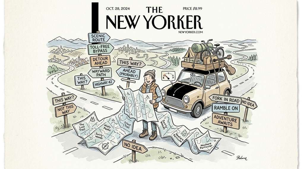
(We define the tuple formally in the next section; this preview shows how all five parts fit together.) Think of the discovery tuple \((S, A, T, f, C)\) like planning a cross-country road trip. The state space \(S\) is the map of every town you could visit. The action space \(A\) is the set of roads you can take from each town. The transition function \(T\) tells you where each road leads (sometimes with uncertainty: a detour or a road closure). The objective \(f\) is your rating of each town (scenery, food, attractions). The constraints \(C\) are your budget, your fuel range, and the requirement to avoid toll roads. Just as a road trip optimizer must know the road network, the fuel costs, and the destination rating to plan an efficient route, a discovery AI must know all five components to search intelligently rather than wandering at random.

3. The Discovery Tuple: \((S, A, T, f, C)\)

Without a shared formal language, teams routinely waste months optimizing the wrong objective or searching a space that omits the actual solution. Making every component of the search explicit turns that silent failure mode into a checklist you can audit before committing resources.

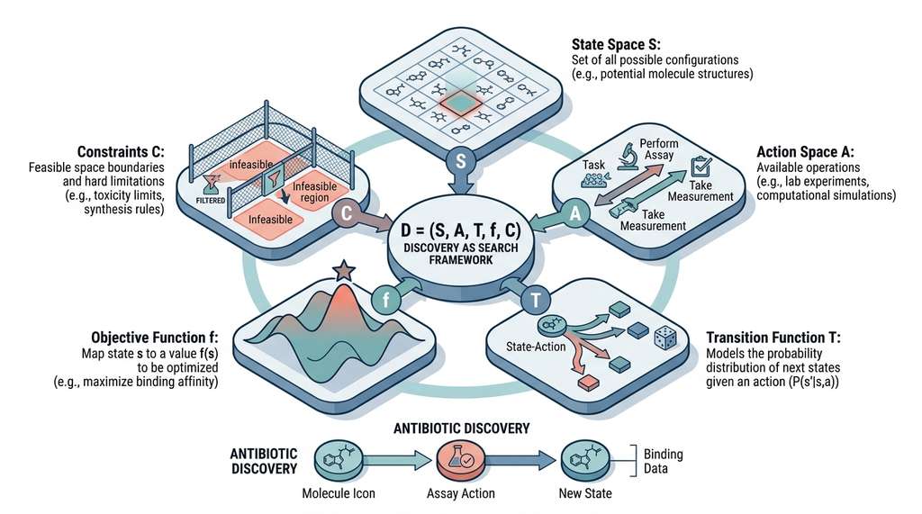
The five-tuple below captures every component of the search process. Figure 1.1 visualizes how the components connect: a state is transformed by an action through the transition function, evaluated by the objective, and filtered by constraints.

A discovery problem is defined by: Figure 1.1.1 illustrates the discovery five-tuple framework.

where:

• \(S\): State space. The set of all possible states the discovery process can occupy. Each state \(s \in S\) encodes everything relevant to the current stage of discovery.
• \(A\): Action space. The set of all actions (experiments, measurements, computations, design choices) available to the discoverer. Actions may depend on the current state: \(A(s) \subseteq A\) gives the actions available in state \(s\).
• \(T\): Transition function. \(T: S \times A \to \Delta(S)\) maps a state-action pair to a probability distribution over next states, where \(\Delta(S)\) denotes the set of all probability distributions over \(S\). The transition is typically stochastic: the same experiment run twice may yield different results due to noise, randomness, or incomplete knowledge.
• \(f\): Objective function. \(f: S \to \mathbb{R}\) (or \(f: S \to \mathbb{R}^k\) for multi-objective discovery) assigns a score to each state. The discoverer seeks states that maximize \(f\).
• \(C\): Constraints. A set of feasibility conditions \(C = \{c_1, c_2, \ldots, c_m\}\) where each \(c_i: S \to \{\text{true}, \text{false}\}\). A state is feasible only if all constraints are satisfied. Constraints encode budgets, safety requirements, physical laws, and ethical boundaries.

Let us ground this abstraction with a concrete example. Consider the problem of discovering a new antibiotic compound.

4. Encoding the Tuple in Python

Abstract mathematics becomes concrete when we write code. The following Python class encodes the discovery tuple as a reusable data structure. We will extend this class throughout the chapter, culminating in the full simulator in Section 1.4.

import numpy as np
from dataclasses import dataclass, field
from typing import Callable, List, Set, Tuple, Optional

@dataclass
class DiscoveryProblem:
    """The five-tuple (S, A, T, f, C) defining a discovery problem.

    For tractability, we represent the state space implicitly:
    states are generated on demand rather than enumerated.
    """
    n_states: int                          # |S|: size of the discrete state space
    n_actions: int                         # |A|: number of available actions
    transition: Callable                   # T(s, a) -> s': state transition
    objective: Callable                    # f(s) -> float: objective value
    constraints: List[Callable]            # [c_i(s) -> bool]: feasibility checks
    rng: np.random.Generator = field(
        default_factory=lambda: np.random.default_rng(42)
    )

    def is_feasible(self, state: int) -> bool:
        """Check whether a state satisfies all constraints."""
        return all(c(state) for c in self.constraints)

    def evaluate(self, state: int) -> Optional[float]:
        """Return objective value if feasible, None otherwise."""
        if not self.is_feasible(state):
            return None
        return self.objective(state)


# --- Example: a simple synthetic discovery landscape ---

def make_synthetic_landscape(n: int = 1000, seed: int = 42):
    """Create a synthetic discovery problem with multi-modal objective.

    The objective has several peaks (local optima) and one global
    optimum, mimicking the rugged fitness landscapes found in
    real discovery problems (e.g., protein fitness landscapes).
    """
    rng = np.random.default_rng(seed)

    # Generate a rugged objective landscape
    x = np.linspace(0, 4 * np.pi, n)
    landscape = (
        np.sin(x) * np.cos(0.5 * x)          # multi-modal base
        + 0.3 * np.sin(5 * x)                 # high-frequency ripple
        + 0.1 * rng.standard_normal(n)         # observation noise
    )

    # Constraints: states in [200, 800] are "feasible"
    # (mimicking a drug-likeness filter)
    def feasibility(s):
        return 200 <= s <= 800

    problem = DiscoveryProblem(
        n_states=n,
        n_actions=n,           # each action = "evaluate state i"
        transition=lambda s, a: a,   # deterministic: action = go to state
        objective=lambda s: landscape[s],
        constraints=[feasibility],
        rng=rng,
    )
    return problem, landscape


problem, landscape = make_synthetic_landscape()
best_state = max(range(200, 801), key=lambda s: landscape[s])
print(f"Search space size: {problem.n_states}")
print(f"Feasible region:   states 200..800 ({601} states)")
print(f"Best feasible state: {best_state}, value: {landscape[best_state]:.4f}")

Search space size: 1000
Feasible region:   states 200..800 (601 states)
Best feasible state: 585, value: 1.5732

Step-Through: Evaluating the Discovery Tuple on a Tiny Landscape

Trace through the synthetic landscape code with a search space of just \(n = 8\) states and a feasible region of states 2 through 5. Suppose the landscape values are:

[0.12, -0.45, 0.88, 1.32, 0.67, -0.11, 0.93, 0.54]

Step 1: Enumerate feasible states: \(\{2, 3, 4, 5\}\). States 0, 1, 6, 7 fail the constraint \(c(s) = (2 \leq s \leq 5)\).
Step 2: Evaluate \(f(s)\) for each feasible state: \(f(2) = 0.88\), \(f(3) = 1.32\), \(f(4) = 0.67\), \(f(5) = -0.11\).
Step 3: Rank by objective: state 3 (1.32) > state 2 (0.88) > state 4 (0.67) > state 5 (\(-0.11\)).
Step 4: Return the best feasible state: \(s^* = 3\) with \(f(s^*) = 1.32\). Note that state 6 has a higher value (0.93) than states 4 and 5, but it is infeasible. Constraints narrow the solution space and can exclude attractive candidates.

5. Multi-Objective Discovery

The synthetic landscape above optimizes a single number, but real discovery problems rarely offer that luxury; a drug candidate that binds perfectly to its target is worthless if it also destroys the patient's liver.

Real discovery problems rarely have a single scalar objective. The antibiotic example above involved four competing criteria. When \(f: S \to \mathbb{R}^k\) with \(k > 1\), we enter the domain of multi-objective optimization. The central concept here is Pareto dominance: state \(s_1\) dominates state \(s_2\) if \(s_1\) is at least as good as \(s_2\) on every objective and strictly better on at least one. The set of non-dominated states forms the Pareto front, where the Pareto front is the boundary of the best achievable trade-offs such that improving one objective necessarily worsens another.

In practice, multi-objective discovery typically proceeds in one of three ways: scalarization (combine objectives into a weighted sum \(f(s) = \sum_i w_i f_i(s)\)), Pareto optimization (find the entire Pareto front and let the human choose), or constraint conversion (optimize one objective while constraining the others to acceptable thresholds). Each approach has trade-offs that we revisit in Chapter 45.

def pareto_front(points: np.ndarray) -> np.ndarray:
    """Find the Pareto-optimal indices for a set of 2D objective vectors.

    Parameters
    ----------
    points : np.ndarray of shape (n, 2)
        Each row is (f1, f2) for one candidate.

    Returns
    -------
    np.ndarray of int
        Indices of Pareto-optimal points.
    """
    n = len(points)
    is_dominated = np.zeros(n, dtype=bool)

    for i in range(n):
        if is_dominated[i]:
            continue
        for j in range(n):
            if i == j or is_dominated[j]:
                continue
            # Check if j dominates i
            if np.all(points[j] >= points[i]) and np.any(points[j] > points[i]):
                is_dominated[i] = True
                break

    return np.where(~is_dominated)[0]


# Generate a two-objective landscape
rng = np.random.default_rng(42)
n_candidates = 200
efficacy = rng.standard_normal(n_candidates)       # objective 1: efficacy
safety = -0.5 * efficacy + rng.standard_normal(n_candidates)  # objective 2: safety (anti-correlated)
points = np.column_stack([efficacy, safety])

front_idx = pareto_front(points)
print(f"Candidates: {n_candidates}")
print(f"Pareto-optimal: {len(front_idx)} ({100*len(front_idx)/n_candidates:.1f}%)")
print(f"Example Pareto point: efficacy={points[front_idx[0], 0]:.2f}, "
      f"safety={points[front_idx[0], 1]:.2f}")

Candidates: 200
Pareto-optimal: 14 (7.0%)
Example Pareto point: efficacy=2.44, safety=-0.14

from pymoo.util.nds.non_dominated_sorting import NonDominatedSorting

# pymoo expects minimization, so negate for maximization
nds = NonDominatedSorting()
fronts = nds.do(-points)  # returns list of arrays, fronts[0] is Pareto-optimal
print(f"Pareto-optimal (pymoo): {len(fronts[0])} points")

6. Why Formalization Matters for AI

With the discovery tuple, search spaces, and multi-objective trade-offs in hand, we have a complete mathematical vocabulary for describing what a discovery problem is; the remaining question is why encoding that vocabulary explicitly is essential for building AI systems that solve these problems.

Why bother with formal tuples when scientists have made discoveries for centuries without them? Because automation requires precision. A human scientist can operate on vague intuitions about what to try next. In practice, an AI system needs an explicit state representation, action space, transition model, objective function, and constraint set; without any one of these, it typically cannot decide what to do or why.

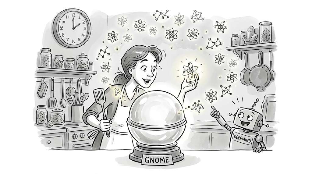
This is not merely an academic exercise. Every real AI discovery system encodes these five components, whether or not its designers use this vocabulary. DeepMind's Graph Networks for Materials Exploration (GNoME) system (Merchant et al., 2023) for crystal structure discovery defines states as crystal structures and actions as structural modifications. A graph neural network serves as the transition function, predicting stability. The objective measures thermodynamic stability via energy above hull (the energy difference between a candidate structure and the most stable known combination of its elements, where lower values indicate greater stability). Constraints enforce charge neutrality and physical realizability. The self-driving laboratories of Chapter 55 make all five components explicit in their control software.

Exercises

1. (Conceptual) Choose a discovery problem from your own field (or one that interests you). Identify all five components of the tuple \((S, A, T, f, C)\). Is the state space discrete, continuous, or mixed? Is the transition function deterministic or stochastic? Write a one-paragraph description in the format of the antibiotic example above.
2. (Coding) Modify the make_synthetic_landscape function to create a landscape with exactly three local optima in the feasible region. Verify your landscape by plotting it with Matplotlib and confirming the number of peaks visually.
3. (Analysis) The Pareto front computation in Listing 1.2 is \(O(n^2)\). Derive the time complexity, then run the code with \(n = 10{,}000\) candidates and measure the wall-clock time. Compare it to the pymoo NonDominatedSorting implementation. What speedup do you observe?