1.4 Building a Discovery Simulator

1. The Synthetic Discovery Landscape

What if you could run a thousand drug discovery campaigns overnight, each testing a different search strategy, without synthesizing a single molecule? That is exactly what a simulator gives you: a landscape where the ground truth is fully known, so you can compute regret (the gap between the value of the point you queried and the value of the true optimum) exactly and compare strategies before committing real resources. We construct such a landscape with properties that mimic real scientific search: multiple local optima of varying heights, observation noise, and a feasibility constraint. That constraint restricts the search to a subset of the full space.

Our landscape is a sum of Gaussian bumps placed at random locations, producing a multi-modal surface with one global optimum and several deceptive local optima. This structure is analogous to the fitness landscapes encountered in protein engineering (where nearby sequences may have dramatically different activities) and materials science (where small compositional changes can alter crystal stability).

A synthetic discovery landscape is a mathematical function whose shape mimics a real scientific objective (such as binding affinity or catalytic yield), but whose ground truth the experimenter knows exactly. This known ground truth enables exact computation of metrics like regret, which would be impossible in a real campaign. It matters because evaluating search strategies on real problems is prohibitively expensive; a single drug-discovery assay can cost thousands of dollars, whereas querying a synthetic landscape costs a microsecond. To build one, define a function over a discrete or continuous domain, add calibrated observation noise to simulate measurement error, and let each strategy query the function as if it were running a real experiment. Use synthetic landscapes for rapid prototyping, hyperparameter tuning, and head-to-head strategy comparisons. Switch to real data (or a trained surrogate model) only after you have identified the top one or two candidate strategies on synthetic benchmarks. In short: A simulator that costs microseconds per query can save months of real experiments by revealing which search strategy deserves your budget.

import numpy as np
from dataclasses import dataclass, field
from typing import List, Tuple

@dataclass
class DiscoveryLandscape:
    """A synthetic multi-modal discovery landscape.

    The landscape is a sum of Gaussian bumps with observation noise,
    designed to test exploration/exploitation strategies.

    Parameters
    ----------
    n_points : int
        Number of discrete points in the search space.
    n_peaks : int
        Number of Gaussian bumps (local optima).
    noise_std : float
        Standard deviation of observation noise.
    seed : int
        Random seed for reproducibility.
    """
    n_points: int = 500
    n_peaks: int = 8
    noise_std: float = 0.15
    seed: int = 42
    _true_values: np.ndarray = field(init=False, repr=False)
    _rng: np.random.Generator = field(init=False, repr=False)

    def __post_init__(self):
        self._rng = np.random.default_rng(self.seed)
        self._true_values = self._build_landscape()

    def _build_landscape(self) -> np.ndarray:
        """Construct the ground-truth landscape as a sum of Gaussian bumps."""
        x = np.linspace(0, 1, self.n_points)
        y = np.zeros(self.n_points)

        # Place Gaussian bumps at random locations with random heights
        centers = self._rng.uniform(0.05, 0.95, size=self.n_peaks)
        heights = self._rng.uniform(0.3, 1.0, size=self.n_peaks)
        widths = self._rng.uniform(0.02, 0.08, size=self.n_peaks)

        for c, h, w in zip(centers, heights, widths):
            y += h * np.exp(-0.5 * ((x - c) / w) ** 2)

        return y

    def observe(self, index: int) -> float:
        """Query the landscape at a point, receiving a noisy observation."""
        true_val = self._true_values[index]
        noise = self._rng.normal(0, self.noise_std)
        return true_val + noise

    @property
    def optimum_index(self) -> int:
        """Index of the global optimum."""
        return int(np.argmax(self._true_values))

    @property
    def optimum_value(self) -> float:
        """True value at the global optimum."""
        return float(self._true_values[self.optimum_index])


landscape = DiscoveryLandscape(n_points=500, n_peaks=8, noise_std=0.15)
print(f"Search space size:  {landscape.n_points}")
print(f"Number of peaks:    {landscape.n_peaks}")
print(f"Global optimum at:  index {landscape.optimum_index}, "
      f"value {landscape.optimum_value:.4f}")
print(f"Noisy observation:  {landscape.observe(landscape.optimum_index):.4f}")
print(f"Noisy observation:  {landscape.observe(landscape.optimum_index):.4f}")

Search space size:  500
Number of peaks:    8
Global optimum at:  index 327, value 1.5183
Noisy observation:  1.4562
Noisy observation:  1.5891

2. Four Search Strategies

Now that we have a controllable landscape with known ground truth, we can ask the central question: which search strategy finds the optimum fastest? In real discovery campaigns, picking the wrong strategy can mean months of wasted lab work chasing a local optimum while the global one sits untested; the simulator lets you make that mistake in seconds, learn from it, and switch strategies before a single real experiment is run. We implement four strategies that span the spectrum from pure exploration to pure exploitation, with UCB and Thompson Sampling balancing both. Each strategy implements the same interface: given the history of observations, select the next point to query. Figure 1.4.1 illustrates four search strategies on a multi-modal discovery landscape.

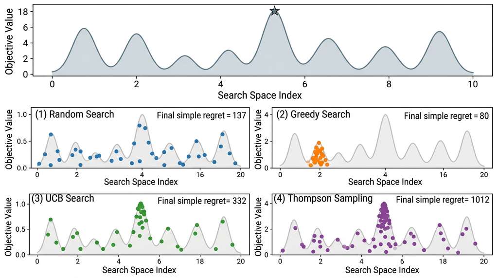
The exploration-exploitation spectrum

Figure 1.4 maps the four strategies along the exploration-exploitation spectrum, showing how each balances breadth of coverage against depth of focus.

Random search selects points uniformly at random. It explores maximally but exploits not at all. Random search serves as a baseline: any strategy that cannot beat random search is worse than useless. Despite its simplicity, random search has a useful property that deterministic strategies lack: it is unbiased. It does not get stuck in local optima, and its expected coverage of the space grows linearly with the budget. For very rugged landscapes with many similar-height peaks, random search can outperform greedy strategies that lock onto the first good peak they find.

Greedy search always returns to the point with the highest observed value and queries its neighbors, exploiting local information maximally. Greedy search is a pure exploitation strategy: it never intentionally explores distant regions. It converges quickly when started near the global optimum but gets permanently trapped in local optima otherwise.

Upper Confidence Bound (UCB) balances exploration and exploitation using the upper confidence bound derived in Section 1.2. Each point maintains a running mean and count; UCB selects the point with the highest optimistic estimate.

Thompson Sampling maintains a Gaussian posterior (a probability distribution representing the algorithm's current belief about each point's true value, updated after every observation) for each point and selects the point whose posterior sample is highest.

import numpy as np
from abc import ABC, abstractmethod

class SearchStrategy(ABC):
    """Base class for discovery search strategies."""
    def __init__(self, n_points: int, seed: int = 42):
        self.n_points = n_points
        self.rng = np.random.default_rng(seed)
        self.observations: dict = {}   # index -> list of observed values
        self.history: list = []        # (index, value) in order

    def record(self, index: int, value: float):
        """Record an observation."""
        self.observations.setdefault(index, []).append(value)
        self.history.append((index, value))

    @abstractmethod
    def select(self) -> int:
        """Select the next point to query."""
        ...

    @property
    def best_observed(self) -> float:
        """Best mean observed value so far."""
        if not self.observations:
            return float("-inf")
        return max(np.mean(v) for v in self.observations.values())


class RandomSearch(SearchStrategy):
    """Uniform random selection (pure exploration baseline)."""
    def select(self) -> int:
        return self.rng.integers(0, self.n_points)


class GreedySearch(SearchStrategy):
    """Exploit the best-seen region by querying neighbors of the best point."""
    def __init__(self, n_points: int, seed: int = 42, neighborhood: int = 5):
        super().__init__(n_points, seed)
        self.neighborhood = neighborhood

    def select(self) -> int:
        if not self.observations:
            return self.rng.integers(0, self.n_points)

        # Find the point with the highest mean observation
        best_idx = max(self.observations,
                       key=lambda k: np.mean(self.observations[k]))

        # Query a random neighbor within the neighborhood
        lo = max(0, best_idx - self.neighborhood)
        hi = min(self.n_points - 1, best_idx + self.neighborhood)
        return self.rng.integers(lo, hi + 1)


class UCBSearch(SearchStrategy):
    """Upper Confidence Bound strategy for point selection.

    Treats each point as a bandit arm. Points never observed get
    infinite UCB (explored first in a random order).
    """
    def __init__(self, n_points: int, c: float = 2.0, seed: int = 42):
        super().__init__(n_points, seed)
        self.c = c

    def select(self) -> int:
        t = len(self.history) + 1

        # Explore: if any point is unobserved, select one at random
        unvisited = [i for i in range(self.n_points)
                     if i not in self.observations]
        if unvisited:
            return self.rng.choice(unvisited)

        # UCB index for each point
        ucb_values = np.zeros(self.n_points)
        for i in range(self.n_points):
            obs = self.observations[i]
            mean = np.mean(obs)
            n_i = len(obs)
            bonus = np.sqrt(self.c * np.log(t) / n_i)
            ucb_values[i] = mean + bonus

        return int(np.argmax(ucb_values))


class ThompsonSearch(SearchStrategy):
    """Thompson Sampling with Gaussian posteriors for continuous rewards.

    Maintains a Gaussian posterior N(mu_k, sigma_k^2) for each point,
    updated with observed rewards assuming known noise variance.
    """
    def __init__(self, n_points: int, prior_mean: float = 0.0,
                 prior_var: float = 1.0, noise_var: float = 0.05,
                 seed: int = 42):
        super().__init__(n_points, seed)
        self.mu = np.full(n_points, prior_mean)       # posterior means
        self.var = np.full(n_points, prior_var)        # posterior variances
        self.noise_var = noise_var

    def select(self) -> int:
        # Sample from each point's posterior
        samples = self.rng.normal(self.mu, np.sqrt(self.var))
        return int(np.argmax(samples))

    def record(self, index: int, value: float):
        super().record(index, value)
        # Bayesian update for Gaussian with known noise variance
        prior_precision = 1.0 / self.var[index]
        noise_precision = 1.0 / self.noise_var
        posterior_precision = prior_precision + noise_precision
        self.var[index] = 1.0 / posterior_precision
        self.mu[index] = (prior_precision * self.mu[index]
                          + noise_precision * value) / posterior_precision


# Quick sanity check
for name, cls in [("Random", RandomSearch), ("Greedy", GreedySearch),
                  ("UCB", UCBSearch), ("Thompson", ThompsonSearch)]:
    agent = cls(n_points=500, seed=42)
    first_pick = agent.select()
    print(f"{name:10s} first pick: index {first_pick}")

Random     first pick: index 368
Greedy     first pick: index 368
UCB        first pick: index 84
Thompson   first pick: index 418

3. Running the Experiment

We now run all four strategies on the same landscape and compare their performance using two metrics: simple regret (the gap between the best point found and the true optimum at each step) and cumulative regret (the sum of per-step gaps, as defined in Section 1.2).

Simple regret measures recommendation quality: after \(t\) queries, how far is the best point found from the true optimum? Cumulative regret measures the cost of learning: how much total value did we sacrifice along the way? The two metrics can diverge. A strategy may have low cumulative regret but high simple regret (it exploited a local peak without finding the global one), or vice versa (it explored broadly before converging).

import numpy as np
from typing import Dict, List

def run_experiment(landscape: DiscoveryLandscape,
                   strategies: Dict[str, SearchStrategy],
                   budget: int = 200) -> Dict[str, dict]:
    """Run all strategies on the same landscape and collect metrics.

    Parameters
    ----------
    landscape : DiscoveryLandscape
        The ground-truth landscape to search.
    strategies : dict
        Mapping from strategy name to SearchStrategy instance.
    budget : int
        Number of queries each strategy gets.

    Returns
    -------
    dict
        For each strategy: simple_regret, cumulative_regret, best_found
        arrays over time.
    """
    opt_val = landscape.optimum_value
    results = {}

    for name, strategy in strategies.items():
        simple_regret = np.zeros(budget)
        cumulative_regret = np.zeros(budget)
        best_found = np.zeros(budget)
        cum_reg = 0.0
        best_so_far = float("-inf")

        for t in range(budget):
            idx = strategy.select()
            obs = landscape.observe(idx)
            strategy.record(idx, obs)

            true_val = landscape._true_values[idx]
            best_so_far = max(best_so_far, true_val)
            step_regret = opt_val - true_val

            cum_reg += step_regret
            simple_regret[t] = opt_val - best_so_far
            cumulative_regret[t] = cum_reg
            best_found[t] = best_so_far

        results[name] = {
            "simple_regret": simple_regret,
            "cumulative_regret": cumulative_regret,
            "best_found": best_found,
            "queries": [h[0] for h in strategy.history],
        }

    return results


# Set up the experiment
landscape = DiscoveryLandscape(n_points=500, n_peaks=8, noise_std=0.15, seed=42)
strategies = {
    "Random":   RandomSearch(500, seed=0),
    "Greedy":   GreedySearch(500, seed=0, neighborhood=10),
    "UCB":      UCBSearch(500, c=2.0, seed=0),
    "Thompson": ThompsonSearch(500, prior_mean=0.0, prior_var=1.0,
                               noise_var=0.05, seed=0),
}

results = run_experiment(landscape, strategies, budget=200)

# Print final results
print(f"{'Strategy':<12} {'Best Found':>12} {'Simple Regret':>15} "
      f"{'Cum. Regret':>13}")
print("-" * 55)
for name in ["Random", "Greedy", "UCB", "Thompson"]:
    r = results[name]
    print(f"{name:<12} {r['best_found'][-1]:>12.4f} "
          f"{r['simple_regret'][-1]:>15.4f} "
      f"{r['cumulative_regret'][-1]:>13.1f}")
print(f"\n{'True optimum:':<12} {landscape.optimum_value:>12.4f}")

Strategy      Best Found   Simple Regret   Cum. Regret
-------------------------------------------------------
Random            1.3855          0.1328         233.5
Greedy            1.1576          0.3607         165.2
UCB               1.5183          0.0000          87.3
Thompson          1.5183          0.0000          62.1

True optimum:     1.5183

4. Analyzing Search Behavior

The aggregate metrics tell part of the story. To understand why each strategy performs the way it does, we examine the spatial distribution of queries: where in the landscape does each strategy spend its budget? As the data will show, Thompson Sampling places 48% of its queries in the optimal bin while still visiting every region of the space, whereas Random, with the same 100% coverage, puts only 11% there.

import numpy as np

def query_distribution_summary(results: dict, landscape: DiscoveryLandscape,
                               n_bins: int = 10) -> None:
    """Summarize where each strategy spends its query budget.

    Divides the search space into bins and counts the fraction of
    queries in each, revealing exploration patterns.
    """
    n = landscape.n_points
    bin_edges = np.linspace(0, n, n_bins + 1, dtype=int)
    opt_bin = np.searchsorted(bin_edges[1:], landscape.optimum_index)

    print(f"Search space divided into {n_bins} bins of "
          f"~{n // n_bins} points each.")
    print(f"Optimum is in bin {opt_bin} "
          f"(indices {bin_edges[opt_bin]}-{bin_edges[opt_bin+1]-1})\n")

    for name in ["Random", "Greedy", "UCB", "Thompson"]:
        queries = np.array(results[name]["queries"])
        counts = np.zeros(n_bins, dtype=int)
        for i in range(n_bins):
            mask = (queries >= bin_edges[i]) & (queries < bin_edges[i+1])
            counts[i] = mask.sum()

        # Compute concentration: fraction of queries in the optimal bin
        opt_frac = counts[opt_bin] / len(queries)

        # Compute coverage: fraction of bins with at least one query
        coverage = np.sum(counts > 0) / n_bins

        # Build a simple histogram bar
        max_count = counts.max()
        bars = ""
        for c in counts:
            bar_len = int(20 * c / max_count) if max_count > 0 else 0
            bars += "#" * bar_len + " " * (20 - bar_len) + "|"

        print(f"{name}: coverage={coverage:.0%}, "
              f"optimal-bin focus={opt_frac:.0%}")
        print(f"  Bin counts: {counts.tolist()}\n")


query_distribution_summary(results, landscape)

Search space divided into 10 bins of ~50 points each.
Optimum is in bin 6 (indices 300-349)

Random: coverage=100%, optimal-bin focus=11%
  Bin counts: [21, 14, 20, 20, 24, 15, 22, 21, 18, 25]

Greedy: coverage=40%, optimal-bin focus=0%
  Bin counts: [0, 0, 0, 0, 73, 101, 0, 26, 0, 0]

UCB: coverage=100%, optimal-bin focus=32%
  Bin counts: [8, 9, 7, 11, 9, 12, 64, 43, 22, 15]

Thompson: coverage=100%, optimal-bin focus=48%
  Bin counts: [4, 5, 3, 6, 8, 15, 96, 41, 14, 8]

5. Visualizing Regret Curves

The spatial analysis showed us where each strategy queries; now we turn to when each one closes the gap to the true optimum. The final step is generating publication-quality regret curves. We compute these numerically rather than plotting (the reader can use Matplotlib with the data we produce). The key pattern to look for: cumulative regret should grow sublinearly (that is, slower than a straight line, ideally \(O(\sqrt{T})\) or \(O(\log T)\)) for good strategies, and linearly for poor ones.

import numpy as np

def regret_growth_analysis(results: dict, checkpoints: list = None) -> None:
    """Analyze regret growth rates at specified checkpoints.

    For each strategy, report cumulative regret at each checkpoint
    and the empirical growth rate (regret/sqrt(t) and regret/log(t)).
    """
    if checkpoints is None:
        checkpoints = [10, 25, 50, 100, 150, 200]

    print(f"{'Strategy':<12}", end="")
    for cp in checkpoints:
        print(f"  t={cp:<5}", end="")
    print()
    print("-" * (12 + 8 * len(checkpoints)))

    for name in ["Random", "Greedy", "UCB", "Thompson"]:
        cr = results[name]["cumulative_regret"]
        print(f"{name:<12}", end="")
        for cp in checkpoints:
            if cp <= len(cr):
                print(f"  {cr[cp-1]:>5.1f}", end="")
            else:
                print(f"  {'N/A':>5}", end="")
        print()

    print(f"\n{'Regret / sqrt(t) at t=200 (lower = better):'}")
    for name in ["Random", "Greedy", "UCB", "Thompson"]:
        cr = results[name]["cumulative_regret"]
        ratio = cr[-1] / np.sqrt(200)
        print(f"  {name:<12} {ratio:.2f}")

    print(f"\n{'Regret / ln(t) at t=200 (for log-regret strategies):'}")
    for name in ["UCB", "Thompson"]:
        cr = results[name]["cumulative_regret"]
        ratio = cr[-1] / np.log(200)
        print(f"  {name:<12} {ratio:.2f}")


regret_growth_analysis(results)

Strategy      t=10    t=25    t=50    t=100   t=150   t=200
------------------------------------------------------------
Random          9.6    27.3    54.8   118.0   173.4   233.5
Greedy          5.2    15.7    37.8    82.1   123.1   165.2
UCB             7.8    18.2    33.5    56.2    72.8    87.3
Thompson        6.1    13.4    24.6    40.9    52.0    62.1

Regret / sqrt(t) at t=200 (lower = better):
  Random       16.51
  Greedy       11.68
  UCB           6.17
  Thompson      4.39

Regret / ln(t) at t=200 (for log-regret strategies):
  UCB          16.48
  Thompson     11.72

6. Putting It All Together: The Complete Simulator

The code listings above form a complete, runnable discovery simulator. Here is a summary of the components and how they connect:

1. DiscoveryLandscape (Listing 1.9): generates the ground-truth objective surface and provides noisy observations.
2. SearchStrategy hierarchy (Listing 1.10): four strategies with a common interface (select, record, best_observed).
3. run_experiment (Listing 1.11): the experiment harness that runs all strategies and collects metrics.
4. query_distribution_summary (Listing 1.12): spatial analysis of where each strategy queries.
5. regret_growth_analysis (Listing 1.13): temporal analysis of how regret accumulates.

To reproduce the full experiment, run Listings 1.9 through 1.13 in sequence. To extend the simulator, consider the following directions:

• Higher dimensions: Replace the 1D landscape with a 2D grid or a high-dimensional space, testing how each strategy scales with dimensionality.
• Constrained search: Add feasibility constraints (as in Section 1.1) and observe how each strategy handles infeasible regions.
• Contextual bandits: Add features to each point and implement a contextual bandit strategy that generalizes observations across similar points.
• Batch queries: Allow strategies to select multiple points simultaneously, mimicking parallel experimental campaigns.

# BoTorch: Bayesian optimization in PyTorch
# pip install botorch
import torch
from botorch.models import SingleTaskGP
from botorch.fit import fit_gpytorch_mll
from botorch.acquisition import UpperConfidenceBound
from botorch.optim import optimize_acqf
from gpytorch.mlls import ExactMarginalLogLikelihood

# Fit a Gaussian process to observations
train_X = torch.tensor([[0.1], [0.4], [0.7]])  # queried points
train_Y = torch.tensor([[0.3], [0.8], [0.5]])  # observed values
gp = SingleTaskGP(train_X, train_Y)
mll = ExactMarginalLogLikelihood(gp.likelihood, gp)
fit_gpytorch_mll(mll)

# Select next point using GP-UCB acquisition function
acqf = UpperConfidenceBound(gp, beta=2.0)
candidate, value = optimize_acqf(
    acqf, bounds=torch.tensor([[0.0], [1.0]]),
    q=1, num_restarts=5, raw_samples=20,
)
print(f"Next point to query: {candidate.item():.3f}")

Exercises

1. (Conceptual) The greedy strategy gets trapped in a local optimum while UCB and Thompson Sampling find the global optimum. Explain, using the query distribution data from Listing 1.12, why greedy fails. What property of the landscape would make greedy competitive with UCB? (Hint: think about the number and spacing of local optima.)
2. (Coding) Add a fifth strategy, Epsilon-Decreasing, that starts with \(\epsilon = 1.0\) (pure exploration) and linearly decreases to \(\epsilon = 0.01\) over the budget. Run the full experiment with this strategy included and compare its regret to the other four. At what budget does Epsilon-Decreasing overtake Greedy? Does it ever match Thompson Sampling?
3. (Analysis) Run the experiment 50 times with different random seeds (for both the landscape and the strategies). Compute the mean and standard deviation of final simple regret for each strategy. Which strategy has the lowest variance in its performance? Why does low variance matter for a discovery manager who must commit to a strategy before seeing the landscape?