Prerequisites
This section requires the Bayesian modeling framework from Section 32.1 and the posterior inference methods from Section 32.2. You should be comfortable with the concept of a posterior distribution and know how to obtain one through Markov chain Monte Carlo (MCMC) or variational inference (VI). Familiarity with information theory (Kullback-Leibler (KL) divergence, entropy) from Appendix A will help with the WAIC derivation. The connection to causal inference (Chapter 31) enriches the model comparison discussion, as causal and statistical models often compete as alternative explanations for the same data.
Scientific discovery is fundamentally about choosing between explanations. Is the relationship linear or quadratic? Does this drug work, or is the effect just noise? Are two populations drawn from the same distribution or different ones? The Bayesian framework provides three complementary tools for these questions: information criteria (WAIC) that estimate out-of-sample predictive accuracy, leave-one-out cross-validation (LOO-CV) that does the same with better finite-sample properties, and Bayes factors that directly compare the marginal evidence for competing hypotheses. Beyond model comparison, this section covers calibration (does the model's stated uncertainty match reality?) and value of information (which experiment should we run next?). Together, these tools turn Bayesian inference from a parameter-estimation method into a complete decision-making framework for scientific discovery.
1. The Widely Applicable Information Criterion (WAIC)
Two climate models fit last century's temperature record equally well, yet one predicts catastrophic warming by 2100 and the other predicts gentle drift; which should a policymaker trust, and how would you know? That question sits at the heart of model comparison: we want to choose the model that will make the best predictions on future data drawn from the same process. The expected log pointwise predictive density (ELPD) measures exactly this:
WAIC is a scoring rule that estimates how well a Bayesian model will predict new, unseen observations, using only the posterior samples you already have. Choosing between models based on training-data fit alone is misleading. A complex model can memorize noise and perform terribly on fresh data. WAIC corrects for this by subtracting a data-driven penalty that grows with effective model complexity. The mechanism works as follows: average each observation's likelihood across all posterior draws to get a raw fit score, then subtract the variance of that log-likelihood across draws. Observations whose likelihood swings wildly across parameter values signal overfitting, so they incur a larger penalty. Use WAIC when you need a quick, posterior-sample-based estimate of predictive performance and your model is reasonably well-specified. Prefer LOO-CV (Section 2) when you need per-observation diagnostics or suspect influential outliers. Prefer Bayes factors (Section 3) when the scientific question concerns which hypothesis is true rather than which model predicts best.
$$\text{ELPD} = \sum_{i=1}^{n} \int p_{\text{true}}(\tilde{y}_i) \log p(\tilde{y}_i \mid D) \, d\tilde{y}_i$$We cannot compute ELPD directly because we do not know the true data-generating distribution \(p_{\text{true}}\). WAIC (Watanabe, 2010) estimates ELPD from the posterior predictive distribution:
$$\widehat{\text{ELPD}}_{\text{WAIC}} = \sum_{i=1}^{n} \log \hat{p}(y_i \mid D) - \sum_{i=1}^{n} V_i$$The first term is the log pointwise predictive density (lppd), where \(\hat{p}(y_i \mid D) = \frac{1}{S} \sum_{s=1}^{S} p(y_i \mid \theta^{(s)})\) averages the likelihood of each observation over posterior samples. The second term \(V_i = \text{Var}_{s}[\log p(y_i \mid \theta^{(s)})]\) is a bias correction that penalizes model complexity: observations that are highly sensitive to the particular parameter values (high variance across posterior samples) contribute more to the penalty. This penalty is the Bayesian analogue of the parameter count in AIC.
Checkpoint
So far: WAIC estimates out-of-sample predictive accuracy from posterior samples by computing the average log-likelihood of each observation across draws (lppd) and then subtracting a variance-based penalty that grows when the model's fit to an observation is sensitive to particular parameter values.
Computing WAIC in Practice
WAIC is computed entirely from posterior samples, making it straightforward to calculate after any MCMC or VI run. Higher WAIC (less negative ELPD) means better expected out-of-sample prediction. In short: the model that best predicts data it has not yet seen is the one that has learned the pattern, not memorized the noise.
2. LOO-CV with Pareto Smoothed Importance Sampling
LOO-CV is the gold standard for estimating out-of-sample prediction: fit the model \(n\) times, each time leaving out one observation, and measure how well the model predicts the left-out point. The LOO-CV estimate of ELPD is:
$$\widehat{\text{ELPD}}_{\text{LOO}} = \sum_{i=1}^{n} \log p(y_i \mid D_{-i})$$where \(D_{-i}\) is the dataset with observation \(i\) removed. Naive LOO-CV requires refitting the model \(n\) times, which is computationally prohibitive for MCMC-based inference. Vehtari, Gelman, and Gabry (2017) showed that Pareto Smoothed Importance Sampling (PSIS) can approximate LOO-CV from a single posterior fit. PSIS reweights the existing posterior samples to approximate the leave-one-out posteriors, then stabilizes the importance weights by fitting a generalized Pareto distribution (a flexible family for modeling the shape of distribution tails) to the largest weights. (For a dataset of 1,000 observations, that is a 1,000x speedup: one posterior fit instead of one thousand.)
The quality of the PSIS approximation is diagnosed by the Pareto \(\hat{k}\) parameter for each observation. If \(\hat{k} < 0.7\), the approximation is reliable. If \(\hat{k} > 0.7\), that observation has too much influence on the posterior, and you need to actually refit the model without that observation (or consider whether the observation is an outlier that warrants investigation, connecting to the anomaly detection methods of Chapter 30).
import pymc as pm
import arviz as az
import numpy as np

# Two competing models for the same data
rng = np.random.default_rng(42)
n = 40
x = rng.uniform(0, 10, size=n)
y_true = 3.0 * np.sin(0.5 * x) + rng.normal(0, 0.8, size=n)

# Model 1: Linear relationship
with pm.Model() as linear_model:
    a = pm.Normal("a", mu=0, sigma=5)
    b = pm.Normal("b", mu=0, sigma=5)
    sigma = pm.HalfNormal("sigma", sigma=3)
    mu = a + b * x
    pm.Normal("y", mu=mu, sigma=sigma, observed=y_true)
    trace_linear = pm.sample(2000, tune=1000, chains=4, random_seed=42)

# Model 2: Sinusoidal relationship (closer to truth)
with pm.Model() as sine_model:
    amp = pm.Normal("amp", mu=0, sigma=5)
    freq = pm.HalfNormal("freq", sigma=2)
    sigma = pm.HalfNormal("sigma", sigma=3)
    mu = amp * pm.math.sin(freq * x)
    pm.Normal("y", mu=mu, sigma=sigma, observed=y_true)
    trace_sine = pm.sample(2000, tune=1000, chains=4, random_seed=42)

# LOO-CV comparison
loo_linear = az.loo(trace_linear, linear_model)
loo_sine = az.loo(trace_sine, sine_model)

# Compare models: ranks by ELPD, reports differences with standard errors
comparison = az.compare(
    {"linear": trace_linear, "sinusoidal": trace_sine},
    ic="loo",
)
print(comparison)

# Check Pareto k diagnostics for the winning model
print(f"\nMax Pareto k (sinusoidal): {loo_sine.pareto_k.values.max():.3f}")
print("Values > 0.7 indicate influential observations needing investigation.")
az.compare function ranks models by ELPD, reports the difference with standard errors, and flags the preferred model. Pareto \(\hat{k}\) diagnostics for each observation are available in loo_sine.pareto_k.The absolute ELPD value of a model is not interpretable on its own; it depends on the scale and number of observations. What matters is the difference in ELPD between models, \(\Delta \text{ELPD} = \text{ELPD}_1 - \text{ELPD}_2\), and whether this difference is large relative to its standard error. A rule of thumb from Vehtari et al.: if \(|\Delta \text{ELPD}| > 4 \cdot \text{SE}\), the difference is decisive. If \(|\Delta \text{ELPD}| < 2 \cdot \text{SE}\), the data cannot distinguish the models. In scientific contexts, the inability to distinguish models is itself a useful finding: it means you need more data or a different experimental design to resolve the question.
3. Bayes Factors
The Bayes factor directly compares the marginal likelihoods (where the marginal likelihood of a model is the probability of the observed data averaged over all parameter values under that model's prior) of two models:
$$\text{BF}_{12} = \frac{p(D \mid M_1)}{p(D \mid M_2)} = \frac{\int p(D \mid \theta_1, M_1) \, p(\theta_1 \mid M_1) \, d\theta_1}{\int p(D \mid \theta_2, M_2) \, p(\theta_2 \mid M_2) \, d\theta_2}$$A Bayes factor of 10 means the data are 10 times more likely under Model 1 than Model 2. Kass and Raftery (1995) provide an interpretation scale: \(\text{BF} > 3.2\) is "substantial" evidence, \(> 10\) is "strong," and \(> 100\) is "decisive." The Bayes factor embodies the Bayesian Occam's razor: a simpler model (narrower prior) that explains the data gets a higher marginal likelihood than a complex model (broad prior) that can explain anything but concentrates less prior mass on the actual observations.
Mental Model
Think of the Bayesian Occam's razor like two weather forecasters competing over a year. Forecaster A (the simple model) always predicts "sunny, 70 to 75 degrees" for Los Angeles. Forecaster B (the complex model) hedges every morning: "somewhere between 30 and 110 degrees, any conditions possible." When the actual temperature is 73, Forecaster A scores well because her narrow prediction concentrated probability right where the observation landed. Forecaster B scores poorly despite technically including 73 in her range, because she spread her probability so thin across all temperatures that the density at 73 is tiny. The Bayes factor measures exactly this: not whether a model can accommodate the data, but how much probability it concentrates on what actually happened. A model that predicts everything predicts nothing.
Common Misconception
A Bayes factor of 10 does not mean there is a 90% probability that Model 1 is correct. The Bayes factor is a likelihood ratio, not a posterior probability. To convert a Bayes factor into a posterior model probability, you must also specify the prior odds: \(\text{posterior odds} = \text{BF} \times \text{prior odds}\). If you started believing both models were equally likely (prior odds = 1), then \(\text{BF}_{12} = 10\) yields posterior odds of 10:1, or roughly 91% for Model 1. But if your prior odds were 1:100 (Model 1 seemed very unlikely before seeing data), the same Bayes factor of 10 gives posterior odds of only 1:10, meaning Model 1 is still the underdog at about 9%. Reporting a Bayes factor without acknowledging that prior model probabilities matter is a common source of overconfident conclusions.
Computing Bayes factors is harder than computing LOO-CV because it requires the marginal likelihood, which is an integral over the entire parameter space. Several approximation methods exist:
- Bridge sampling (Meng and Wong, 1996): uses an auxiliary "bridge" distribution to connect posterior samples from both models. Available in the
bridgesamplingR package and Python implementations. - Savage-Dickey ratio: for nested models where one model fixes a parameter \(\psi = \psi_0\) that the other estimates freely, the Bayes factor equals the ratio of the posterior to the prior density at \(\psi_0\). Elegant when applicable.
- Harmonic mean estimator: tempting but numerically unstable; the variance is often infinite. Avoid in practice.
A neuroscientist measures brain activation in response to a stimulus. Model 1 says the effect size \(\delta\) is nonzero; Model 2 says \(\delta = 0\) (no effect). These are nested: Model 2 is Model 1 with \(\delta\) fixed at zero. The Savage-Dickey ratio gives the Bayes factor as \(\text{BF}_{20} = p(\delta = 0 \mid D) / p(\delta = 0)\), the ratio of the posterior density at zero to the prior density at zero. If the posterior has moved mass away from zero, the denominator exceeds the numerator, and \(\text{BF}_{20} < 1\), meaning the data favor a nonzero effect. This is computed from a single posterior fit, with no refitting needed.
import pymc as pm
import numpy as np
from scipy.stats import norm, gaussian_kde

# Simulated experiment: small effect with moderate noise
rng = np.random.default_rng(42)
effect_true = 0.35     # small but real effect
data = rng.normal(effect_true, 1.0, size=25)

with pm.Model() as effect_model:
    delta = pm.Normal("delta", mu=0, sigma=1)     # prior centered at 0
    sigma = pm.HalfNormal("sigma", sigma=2)
    pm.Normal("obs", mu=delta, sigma=sigma, observed=data)
    trace = pm.sample(4000, tune=2000, chains=4, random_seed=42)

# Savage-Dickey ratio: BF for delta = 0 (null) vs delta != 0
posterior_samples = trace.posterior["delta"].values.flatten()
prior_at_zero = norm.pdf(0, loc=0, scale=1)  # Normal(0,1) density at 0

kde = gaussian_kde(posterior_samples)
posterior_at_zero = kde.evaluate(0.0)[0]

bf_null = posterior_at_zero / prior_at_zero
bf_alt = 1.0 / bf_null

print(f"Prior density at delta=0:     {prior_at_zero:.4f}")
print(f"Posterior density at delta=0:  {posterior_at_zero:.4f}")
print(f"BF (null vs alternative):     {bf_null:.3f}")
print(f"BF (alternative vs null):     {bf_alt:.3f}")
# BF_alt > 3 suggests substantial evidence for a nonzero effect
4. WAIC vs. LOO-CV vs. Bayes Factors
These three approaches answer subtly different questions, and choosing among them depends on the scientific context, as summarized in Table 32.3:
| Criterion | Question Answered | Sensitivity to Priors | Best For |
|---|---|---|---|
| WAIC | Which model predicts best? | Low (data-dominated) | Routine model selection |
| LOO-CV (PSIS) | Which model predicts best? | Low (data-dominated) | Same as WAIC, better diagnostics |
| Bayes factor | Which hypothesis is more likely? | High (prior-dependent) | Hypothesis testing, theory comparison |
In practice, LOO-CV is the default recommendation (Vehtari et al., 2017). It is easy to compute from posterior samples, provides per-observation diagnostics, and answers the practical question of which model predicts better. Bayes factors are appropriate when the scientific question is genuinely about comparing theories (does this effect exist? is this physical law the correct one?) rather than about prediction.
ArviZ handles all three criteria through a unified interface. az.loo(trace)
computes PSIS-LOO-CV. az.waic(trace) computes WAIC. az.compare({"m1":
trace1, "m2": trace2}) ranks any number of models by either criterion, reports
ELPD differences with standard errors, and produces publication-quality comparison
plots with az.plot_compare. The entire comparison pipeline, which would
require several hundred lines of manual code, is reduced to roughly 5 lines. ArviZ
also provides az.plot_loo_pit for calibration checking (see below).
5. Calibration: Does Your Uncertainty Match Reality?
Selecting the best model is only half the job; you also need to verify that the winning model's stated uncertainty is trustworthy.
A model that reports 95% credible intervals should contain the true value 95% of the time. If it does, the model is well-calibrated. If 95% intervals contain the truth only 80% of the time, the model is overconfident (reporting narrower uncertainty than it should). If they contain the truth 99% of the time, the model is underconfident (wasting information by reporting wider uncertainty than necessary).
The standard tool for checking calibration is the probability integral transform (PIT). For each observation \(y_i\), compute the posterior predictive cumulative distribution function (CDF), where the CDF at a value is the probability that a new draw from the model would fall at or below that value, evaluated at \(y_i\): \(u_i = P(Y_i \leq y_i \mid D)\). If the model is well-calibrated, these PIT values should be uniformly distributed on \([0, 1]\) (because under a correct model, the probability of an observation falling below any given quantile is, by definition, equal to that quantile). Deviations from uniformity diagnose specific problems: a U-shaped PIT histogram indicates that the model's predictive intervals are too narrow (observations land in the tails more often than predicted), and an inverse U-shape indicates that the model's predictive intervals are too wide (observations cluster near the center).
import arviz as az
import numpy as np

def check_calibration(trace, model, observed, var_name="y"):
    """Check calibration via PIT histogram and coverage analysis.

    Args:
        trace: InferenceData from MCMC sampling
        model: PyMC model context
        observed: array of observed values
        var_name: name of the observed variable in the model
    Returns:
        pit_values: array of PIT values for each observation
    """
    with model:
        ppc = pm.sample_posterior_predictive(trace, random_seed=42)

    # Compute PIT values: fraction of posterior predictive samples <= observed
    ppc_samples = ppc.posterior_predictive[var_name].values
    ppc_flat = ppc_samples.reshape(-1, len(observed))  # (total_draws, n_obs)

    pit_values = np.mean(ppc_flat <= observed[np.newaxis, :], axis=0)

    # Check coverage at multiple nominal levels
    print("Calibration report:")
    for level in [0.50, 0.80, 0.90, 0.95]:
        alpha = 1 - level
        lower = np.quantile(ppc_flat, alpha / 2, axis=0)
        upper = np.quantile(ppc_flat, 1 - alpha / 2, axis=0)
        coverage = np.mean((observed >= lower) & (observed <= upper))
        gap = abs(coverage - level)
        status = "GOOD" if gap < 0.05 else "WARN" if gap < 0.10 else "BAD"
        print(f"  {level*100:.0f}% interval: coverage = {coverage:.3f} [{status}]")

    # ArviZ provides the PIT plot as a one-liner
    az.plot_loo_pit(idata=trace, y=var_name)

    return pit_values
plot_loo_pit provides the same analysis as a publication-quality plot.
Standard Bayesian credible intervals are calibrated only when the model is
well-specified and the inference algorithm converges correctly. Simulation-Based
Calibration (SBC), formalized by Talts et al. (2018), checks both at once by
repeatedly simulating data from the prior, running inference, and verifying that the
resulting rank statistics are uniform. In 2023, Sailynoja, Burkner, and Vehtari
extended SBC into a practical toolkit with their paper "Graphical test for discrete
uniformity and its applications in goodness of fit evaluation and multiple sample
comparison" (Statistics and Computing, 2022/2023), providing powerful visual
diagnostics (empirical CDF (ECDF) difference plots) that detect subtle inference failures traditional
trace plots miss. The ArviZ library now integrates SBC workflows via
az.plot_ecdf and related utilities. Separately, Fong and Holmes's
conformal Bayesian prediction framework continues to gain traction,
with Angelopoulos and Bates (2023) publishing "Conformal Prediction: A Gentle
Introduction" (Foundations and Trends in Machine Learning), which unifies
conformal calibration methods and demonstrates their application to Bayesian models
in drug discovery and materials science, providing distribution-free coverage
guarantees even when the Bayesian model is misspecified.
6. Value of Information: Which Experiment Should We Run Next?
Once calibration confirms that the model's uncertainty reflects reality, a natural next question arises: where should we look to reduce that uncertainty most efficiently?
The expected information gain (EIG) answers a question that is central to scientific discovery: given our current knowledge (the posterior), which possible experiment would teach us the most? The EIG of an experiment \(\xi\) is the expected reduction in posterior entropy:
$$\text{EIG}(\xi) = \mathbb{E}_{p(y \mid \xi, D)} \left[ \text{KL}\!\left( p(\theta \mid y, \xi, D) \;\|\; p(\theta \mid D) \right) \right]$$This is the expected KL divergence (a non-negative measure of how much one probability distribution differs from another; zero only when the two distributions are identical) between the posterior we would have after observing the outcome \(y\) and the posterior we have now. Experiments with high EIG are those whose outcomes would substantially change our beliefs, regardless of what those outcomes turn out to be.
Computing EIG exactly requires marginalizing over all possible experimental outcomes, an integral over the data space. For models that support sampling from the posterior predictive distribution (the distribution of new observations implied by the posterior over parameters), Monte Carlo provides a practical estimator:
import numpy as np
from scipy.stats import norm

def expected_information_gain(
    posterior_samples, likelihood_fn, design_points, n_mc=200, rng=None
):
    """Estimate expected information gain for candidate experimental designs.

    Uses the nested Monte Carlo estimator of Myung et al. (2013).

    Args:
        posterior_samples: (n_post, n_params) draws from current posterior
        likelihood_fn: callable (theta, x_design) -> (mean, std) of observation
        design_points: array of candidate experimental conditions
        n_mc: number of synthetic observations per design point
        rng: numpy random generator
    Returns:
        eig: array of EIG estimates, one per design point
    """
    if rng is None:
        rng = np.random.default_rng(0)
    n_post = len(posterior_samples)
    eig = np.zeros(len(design_points))

    for d_idx, x_d in enumerate(design_points):
        mi_samples = []

        for _ in range(n_mc):
            # 1. Draw a "true" theta from the posterior
            idx = rng.integers(n_post)
            theta_star = posterior_samples[idx]
            mu_star, sigma_star = likelihood_fn(theta_star, x_d)

            # 2. Simulate an observation under theta_star
            y_sim = rng.normal(mu_star, sigma_star)

            # 3. Evaluate log p(y_sim | theta) for all posterior samples
            log_likes = np.array([
                norm.logpdf(y_sim, *likelihood_fn(theta, x_d))
                for theta in posterior_samples
            ])

            # 4. Log marginal: log (1/S) sum_s p(y_sim | theta_s)
            log_marginal = np.logaddexp.reduce(log_likes) - np.log(n_post)

            # 5. Log conditional: log p(y_sim | theta_star)
            log_cond = norm.logpdf(y_sim, mu_star, sigma_star)

            mi_samples.append(log_cond - log_marginal)

        eig[d_idx] = np.mean(mi_samples)

    return eig

# Example: which temperature to measure next for a reaction rate study?
candidate_temps = np.linspace(250, 500, 50)  # Kelvin
# eig = expected_information_gain(posterior_samples, arrhenius_likelihood, candidate_temps)
# optimal_temp = candidate_temps[np.argmax(eig)]
# print(f"Most informative next measurement: {optimal_temp:.0f} K")
Expected information gain has a useful theoretical property: it tends to balance exploring regions of parameter space where uncertainty is high against exploiting regions where the model predicts interesting phenomena. A design point in a well-characterized region has low EIG because no plausible outcome would change our beliefs much. A design point in an uncertain region has high EIG because many different outcomes are plausible, and each would update the posterior substantially. This is the same exploration-exploitation trade-off that appears in reinforcement learning and Bayesian optimization (Chapter 45), but derived from first principles rather than imposed as a heuristic.
7. The Decision-Theoretic Discovery Cycle
The complete Bayesian discovery cycle integrates model building, comparison, calibration, and experimental design into a coherent loop. Figure 32.4 illustrates the six stages of this cycle, showing how each stage feeds into the next. Figure 32.3.1 illustrates Bayesian decision-theoretic discovery cycle.
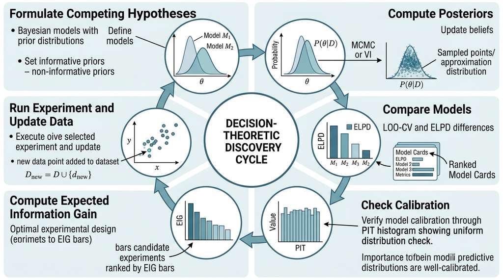
- Formulate competing hypotheses as Bayesian models (Section 32.1).
- Compute posteriors for each model (Section 32.2).
- Compare models using LOO-CV to identify the best-supported hypothesis.
- Check calibration to verify that the winning model's uncertainty is trustworthy.
- Compute EIG to determine the most informative next experiment.
- Run the experiment, update the data, and return to step 2.
This loop is the quantitative backbone of the automated experiment design systems in Chapter 46 and the self-driving laboratories of Chapter 55, where it runs autonomously: a robot executes experiments while a Bayesian model decides what to try next.
Exercise 32.3.1
You have two PyMC models fitted to the same 60-observation dataset. ArviZ reports
az.compare results: Model A has ELPD = -82.3, Model B has ELPD = -85.1,
and the standard error of the difference is 1.8. Meanwhile, a Savage-Dickey Bayes
factor computation gives BF(A vs B) = 0.4, favoring Model B. Which model does LOO-CV
prefer, which does the Bayes factor prefer, and can both be correct simultaneously?
Justify your answer by explaining what each criterion actually measures.
Hint
LOO-CV ranks by predictive accuracy on held-out data and is largely insensitive to priors. The Bayes factor ranks by marginal likelihood, which is heavily influenced by the prior. A model with diffuse priors can predict well (high ELPD) yet score a low marginal likelihood because the prior spread probability mass over regions the data never visited. Check whether the ELPD difference (2.8) exceeds 2 times the SE (3.6) to assess decisiveness.
Step-Through: Computing WAIC by Hand
Trace through the WAIC calculation with a tiny example: 3 observations and 4 posterior samples.
Data: \(y = [1.0,\; 2.5,\; 4.0]\). Posterior samples of \(\theta\) yield these log-likelihoods \(\log p(y_i \mid \theta^{(s)})\):
Observation \(y_1{=}1.0\): [-1.2, -1.0, -1.3, -1.1] → $\hat{p}(y_1 \mid D) = \frac{1}{4}(e^{-1.2} + e^{-1.0} + e^{-1.3} + e^{-1.1}) = \frac{1}{4}(0.301 + 0.368 + 0.272 + 0.333) = 0.319$ → \(\log \hat{p} = -1.143\). Variance of log-likes: \(V_1 = \text{Var}([-1.2, -1.0, -1.3, -1.1]) = 0.0125\).
Observation \(y_2{=}2.5\): [-0.8, -0.9, -0.7, -0.85] → \(\hat{p} = \frac{1}{4}(0.449 + 0.407 + 0.497 + 0.427) = 0.445\) → \(\log \hat{p} = -0.810\). \(V_2 = \text{Var}([-0.8, -0.9, -0.7, -0.85]) = 0.00563\).
Observation \(y_3{=}4.0\): [-2.0, -1.5, -2.3, -1.8] → \(\hat{p} = \frac{1}{4}(0.135 + 0.223 + 0.100 + 0.165) = 0.156\) → \(\log \hat{p} = -1.858\). \(V_3 = \text{Var}([-2.0, -1.5, -2.3, -1.8]) = 0.0892\).
WAIC: lppd \(= -1.143 + (-0.810) + (-1.858) = -3.811\). Penalty \(= 0.0125 + 0.00563 + 0.0892 = 0.107\). $\widehat{\text{ELPD}}_{\text{WAIC}} = -3.811 - 0.107 = -3.918$. Notice that $y_3$ contributes most of the penalty (0.089 of 0.107): its likelihood swings the most across posterior samples, signaling that the model is most uncertain about that observation.
Real-World Application: Drug Discovery at Novartis
Novartis's Bayesian clinical trial platform uses LOO-CV and WAIC to compare dose-response models (linear, Emax, sigmoidal Emax) during Phase II studies. Rather than committing to a single functional form before unblinding, the team fits all candidate models to accumulating data, ranks them by PSIS-LOO, and uses model-averaged posterior predictions to recommend the dose for Phase III. This approach, described in their 2020 Statistics in Medicine publication, reportedly reduced the rate of Phase III dose-selection failures by letting the data, not tradition, choose the dose-response shape.
Lab: LOO-CV Showdown on Real Climate Data
Goal: Use LOO-CV to decide whether global temperature anomalies (1880 to present) are better described by a linear trend, a quadratic trend, or a changepoint model.
Tools: Python with PyMC (v5+), ArviZ, pandas, and matplotlib. Download
the NASA GISTEMP global mean land-ocean temperature index CSV from
data.giss.nasa.gov (or use pd.read_csv on the direct URL).
Procedure (25 minutes):
(1) Load the annual anomaly series and standardize the year variable to zero mean.
(2) Fit three PyMC models: linear (\(\mu = a + b \cdot \text{year}\)), quadratic
(\(\mu = a + b \cdot \text{year} + c \cdot \text{year}^2\)), and a changepoint model
where slope changes at an estimated year \(\tau\) (use a continuous approximation with
a logistic switch). Sample 2000 draws, 4 chains each.
(3) Run az.compare with ic="loo" and print the ranking.
(4) Inspect Pareto \(\hat{k}\) diagnostics for the best model; identify any
observations with \(\hat{k} > 0.7\).
What to vary: Try restricting the dataset to 1950-present vs. 1880-present. Does the best model change? Try widening vs. narrowing the priors on the changepoint year \(\tau\).
What to observe: Which model wins, by how many ELPD units? Do the high-\(\hat{k}\) years correspond to known volcanic eruptions or El Nino events? Does the changepoint model's estimated \(\tau\) align with the commonly cited acceleration around 1970?
Sometimes LOO-CV reports that two competing models predict equally well. This is not a failure of the method; it is a genuine scientific finding: the available data cannot distinguish between the hypotheses. In pharmaceutical research, this often means that a cheaper, simpler assay would be sufficient (the complex model adds no predictive value). In physics, it might mean that a proposed extension to the standard model is neither confirmed nor ruled out by current accelerator data. The EIG calculation then tells you exactly which experiment would break the tie.
Try It: Compare Three Regression Models with LOO-CV
Build a complete model comparison pipeline on your laptop using PyMC and ArviZ.
Step 1. Generate 50 data points from a quadratic model:
y = 1.0 + 0.8*x + 0.3*x**2 + noise where x is uniformly
spaced on [-3, 3] and noise is Normal(0, 1). Use numpy only.
Step 2. Define three PyMC models for this data: (a) linear
(mu = a + b*x), (b) quadratic (mu = a + b*x + c*x**2),
and (c) cubic (mu = a + b*x + c*x**2 + d*x**3). Use Normal(0, 5)
priors for all coefficients and HalfNormal(sigma=3) for the noise. Sample 2000
draws with 4 chains for each model.
Step 3. Run az.compare({"linear": trace1, "quadratic": trace2,
"cubic": trace3}, ic="loo") and print the resulting DataFrame. Verify that the
quadratic model ranks first and check whether the ELPD difference to the cubic model
is within 2 standard errors (meaning the data cannot distinguish them).
Step 4. Inspect the Pareto \(\hat{k}\) values for the winning model
with az.loo(trace2, quadratic_model).pareto_k.values.max(). If any value
exceeds 0.7, identify which observation is problematic and consider whether it is an
outlier.
Step 5. Generate a calibration check for the winning model: run
pm.sample_posterior_predictive, compute empirical coverage at the 50%,
80%, and 95% levels, and compare to the nominal values. A well-calibrated model
should show coverage within 5 percentage points of each target. Plot the PIT
histogram with az.plot_loo_pit and confirm it looks approximately
uniform.
Exercises
- (Conceptual) A Bayes factor of 0.5 for Model A versus Model B means the data moderately favor Model B. But a LOO-CV comparison shows Model A has higher ELPD. Explain how these two criteria can disagree. Which should you trust, and under what circumstances? Hint: consider the role of priors in each criterion.
-
(Coding) Generate data from a quadratic model \(y = 2 + 0.5x + 0.1x^2 + \epsilon\) with \(n = 30\) points and \(\epsilon \sim \text{Normal}(0, 1)\). Fit three PyMC models (linear, quadratic, cubic) and compare them using
az.comparewith LOO-CV. How does the ranking change as you increase \(n\) to 100 and 500? At what sample size does LOO-CV reliably identify the quadratic model as best? - (Analysis) Using the EIG estimation function from this section, design an optimal 5-point experiment for a simple linear regression model \(y = a + bx + \epsilon\). Start with a prior \(a \sim \text{Normal}(0, 10)\), \(b \sim \text{Normal}(0, 10)\), \(\sigma = 1\), and candidate design points \(x \in \{-5, -4, \ldots, 4, 5\}\). After each observation (simulated from the true model with \(a=1, b=2\)), update the posterior and recompute EIG. Where does the optimal design place its points, and how does this compare to classical D-optimal design (where D-optimality selects design points that maximize the determinant of the Fisher information matrix, concentrating measurements at the extremes of the design space)?
What's Next
The complete Bayesian toolkit now spans model specification, posterior inference, model comparison, calibration, and experimental design. In Section 32.4: Building a Bayesian Discovery Model, all of these pieces come together in a complete recipe: two competing hypotheses about enzyme kinetics, full PyMC inference with the No-U-Turn Sampler (NUTS), LOO-CV model comparison, expected information gain for the next experiment, and integration with the Discovery Workbench.
Bibliography
The foundational paper on PSIS-LOO-CV with Pareto \(\hat{k}\) diagnostics.
The original WAIC paper deriving the criterion from singular learning theory.
The standard reference for interpreting and computing Bayes factors in scientific hypothesis testing.
The library providing LOO-CV, WAIC, PIT calibration checks, and model comparison plots used throughout this section.
Tutorial on Bayesian adaptive experimental design, providing the nested Monte Carlo estimator for EIG used in this section.
Survey of computational methods for Bayesian experimental design connecting EIG to classical optimal design theory.