A robotic chemist has fifteen reagent slots, a twenty-step budget, and one night to find a high-yield catalyst; every experiment it runs reshapes what it should try next. Bayesian optimization and evolutionary methods treat the objective as a static function: evaluate candidates, observe fitness, repeat. But problems like that robotic chemist's are inherently sequential. A retrosynthesis planner must choose a sequence of reactions. A materials screening campaign allocates budget across multiple stages, each informed by the last. These are sequential decision problems, and reinforcement learning (RL) provides the mathematical framework to solve them. This section develops policy gradient methods and actor-critic architectures, then shows when RL outperforms static optimization and when it does not.
1. Discovery as a Markov Decision Process
A Markov Decision Process (MDP) is defined by the tuple \((\mathcal{S}, \mathcal{A}, P, R, \gamma)\):
An MDP models any situation where an agent makes sequential decisions under uncertainty, receiving feedback after each step. It matters because it transforms vague notions of "planning" into a precise optimization problem with provable solution methods. Given the state, transition, and reward structure, algorithms compute the decision rule (policy) that maximizes long-term cumulative reward. The core mechanism is the Bellman equation, which splits a multi-step plan's value into the immediate reward plus the discounted value of the next state. This decomposition enables dynamic programming or gradient-based solutions. Use an MDP formulation (and therefore RL) instead of single-shot optimization when earlier decisions affect later options. If each evaluation is independent, simpler methods like Bayesian optimization or evolutionary search are more sample-efficient.
- States \(\mathcal{S}\): the current state of knowledge (observed data, remaining budget, intermediate compounds synthesized so far).
- Actions \(\mathcal{A}\): the set of possible next experiments, reactions, or measurements.
- Transition dynamics \(P(s' \mid s, a)\): how the state evolves after taking action \(a\) in state \(s\). In discovery, this includes both the deterministic part (budget decreases, data accumulates) and the stochastic part (experiment outcomes are noisy).
- Reward \(R(s, a, s')\): the immediate value of the transition. This might be the activity of a newly synthesized compound, the information gained from a measurement, or a penalty for resource consumption.
- Discount factor \(\gamma \in [0, 1]\): how much the agent values future rewards relative to immediate ones.
The goal is to find a policy \(\pi(a \mid s)\) (a distribution over actions given the current state) that maximizes the expected cumulative reward:
$$J(\pi) = \mathbb{E}_{\tau \sim \pi}\left[\sum_{t=0}^{T} \gamma^t R(s_t, a_t, s_{t+1})\right]$$where \(\tau = (s_0, a_0, s_1, a_1, \ldots)\) is a trajectory sampled by following policy \(\pi\) in the MDP.
The critical difference between RL and Bayesian optimization (BO) is that RL optimizes a policy (a decision rule), not a single point. The policy maps states to actions, meaning it adapts to what has been observed so far. BO's acquisition function does something similar (it conditions on all past data), but RL explicitly models the sequential structure and can learn long-horizon strategies that BO cannot represent.
Mapping a discovery campaign to an MDP requires careful state design. Table 45.1 shows three example mappings.
| Campaign | State \(s\) | Action \(a\) | Reward \(R\) | Horizon \(T\) |
|---|---|---|---|---|
| Drug screening | Tested compounds, assay results, budget remaining | Choose next compound to test | Activity of tested compound | Budget / cost-per-test |
| Retrosynthesis | Current molecule, available reagents | Choose reaction template | +1 if target reached, 0 otherwise | Max synthesis steps |
| Robotic lab | Instrument states, sample queue, results so far | Schedule next instrument action | Information gain from measurement | Shift duration |
2. The Policy Gradient Theorem
The MDP formulation raises a core question: how to find the policy that maximizes cumulative reward.
If the agent cannot estimate how a small change to its decision rule will affect cumulative reward, it is reduced to random trial and error, wasting every experiment in a budget-limited campaign. The policy gradient theorem solves exactly this problem, providing an unbiased gradient signal that turns sequential discovery into tractable optimization.
We parameterize the policy as \(\pi_\theta(a \mid s)\) using a neural network with parameters \(\theta\). The policy gradient theorem (Sutton et al., 1999) gives us the gradient of the expected return with respect to \(\theta\):
$$\nabla_\theta J(\theta) = \mathbb{E}_{\tau \sim \pi_\theta}\left[\sum_{t=0}^{T} \nabla_\theta \log \pi_\theta(a_t \mid s_t)\, G_t\right]$$where \(G_t = \sum_{k=t}^{T} \gamma^{k-t} R_k\) is the return from time step \(t\). This expression uses the log-derivative trick: because \(\nabla_\theta \pi_\theta = \pi_\theta \nabla_\theta \log \pi_\theta\), we can estimate the gradient by sampling trajectories under \(\pi_\theta\) and weighting each action's log-probability by the return that followed it. Actions that led to high returns get reinforced (their probability increases); actions that led to low returns get suppressed. In short: weight each decision by the outcome it produced, then nudge the policy toward decisions that paid off.
2.1 REINFORCE
The simplest policy gradient algorithm, REINFORCE (Williams, 1992), directly applies the policy gradient theorem using Monte Carlo estimates (where the return \(G_t\) is computed from a complete sampled trajectory rather than bootstrapped from a value function) of \(G_t\):
import torch
import torch.nn as nn
import torch.optim as optim
from torch.distributions import Categorical
import numpy as np

class PolicyNetwork(nn.Module):
    """Simple policy network for discrete action spaces."""

    def __init__(self, state_dim: int, n_actions: int, hidden: int = 64):
        super().__init__()
        self.net = nn.Sequential(
            nn.Linear(state_dim, hidden),
            nn.ReLU(),
            nn.Linear(hidden, hidden),
            nn.ReLU(),
            nn.Linear(hidden, n_actions),
        )

    def forward(self, state: torch.Tensor) -> Categorical:
        logits = self.net(state)
        return Categorical(logits=logits)


def reinforce(
    env,
    policy: PolicyNetwork,
    n_episodes: int = 1000,
    lr: float = 1e-3,
    gamma: float = 0.99,
) -> list:
    """Train a policy using REINFORCE with baseline subtraction.

    Parameters
    ----------
    env : environment with reset() -> state, step(action) -> (state, reward, done)
    policy : PolicyNetwork
    n_episodes : int
    lr : float
    gamma : float

    Returns
    -------
    episode_returns : list of float
        Total return per episode.
    """
    optimizer = optim.Adam(policy.parameters(), lr=lr)
    baseline = 0.0  # Running average baseline
    episode_returns = []

    for episode in range(n_episodes):
        state = env.reset()
        log_probs = []
        rewards = []

        # Collect a trajectory
        done = False
        while not done:
            state_t = torch.FloatTensor(state)
            dist = policy(state_t)
            action = dist.sample()
            log_probs.append(dist.log_prob(action))

            state, reward, done, _ = env.step(action.item())
            rewards.append(reward)

        # Compute discounted returns
        returns = []
        G = 0.0
        for r in reversed(rewards):
            G = r + gamma * G
            returns.insert(0, G)
        returns = torch.FloatTensor(returns)

        # Baseline subtraction reduces variance
        episode_return = returns[0].item()
        baseline = 0.99 * baseline + 0.01 * episode_return
        returns = returns - baseline

        # Policy gradient update
        loss = -torch.stack([lp * G for lp, G in zip(log_probs, returns)]).sum()
        optimizer.zero_grad()
        loss.backward()
        optimizer.step()

        episode_returns.append(episode_return)

return episode_returnsenv.step() to return five values (obs, reward, terminated, truncated, info) instead of four. For current Gymnasium versions, replace done with terminated or truncated. The baseline subtraction does not change the expected gradient (it is a constant shift) but dramatically reduces variance, making learning more stable. The policy network outputs a categorical distribution over discrete actions.REINFORCE is simple but suffers from high variance: each gradient estimate depends on the return of an entire trajectory, and trajectories vary widely. Two techniques reduce this variance: baseline subtraction (implemented above) and using a learned value function as the baseline, which leads us to actor-critic methods.
3. Actor-Critic Methods
An actor-critic architecture maintains two networks: the actor \(\pi_\theta(a \mid s)\) (the policy) and the critic \(V_\phi(s)\) (a value function that estimates the expected return from state \(s\)). The critic replaces the Monte Carlo return \(G_t\) with a lower-variance estimate, the advantage. Figure 45.3.1 illustrates Actor-Critic Architecture for Sequential Discovery.
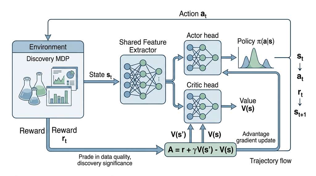
The advantage measures how much better action \(a_t\) was compared to the average action from state \(s_t\). The policy gradient becomes:
$$\nabla_\theta J \approx \mathbb{E}\left[\sum_t \nabla_\theta \log \pi_\theta(a_t \mid s_t)\, A(s_t, a_t)\right]$$Figure 45.3 illustrates how the actor and critic interact during training. The shared feature extractor feeds both heads, and the environment closes the loop by returning rewards and next states.
Mental Model
Think of the advantage function like a restaurant review that accounts for expectations. If you visit a restaurant in a neighborhood where most places are mediocre (low \(V_\phi(s)\)), even a decent meal produces a positive "advantage" (it exceeded the baseline). But the same meal at a restaurant in a world-class food district (high \(V_\phi(s)\)) produces a negative advantage, because it fell below what you expected from that location. The critic learns these neighborhood expectations, and the actor uses the relative surprise (positive or negative) to adjust its choices. Without this calibration, the agent would treat every good meal the same regardless of context, learning much more slowly.
The critic is trained to minimize the squared temporal-difference (TD) error (the gap between the critic's current value estimate and a one-step-ahead bootstrap target, used as a training signal to improve the critic): \(\mathcal{L}_\text{critic} = \mathbb{E}[(R_t + \gamma V_\phi(s_{t+1}) - V_\phi(s_t))^2]\).
class ActorCritic(nn.Module):
    """Combined actor-critic network with shared feature extractor."""

    def __init__(self, state_dim: int, n_actions: int, hidden: int = 128):
        super().__init__()
        # Shared feature layers
        self.shared = nn.Sequential(
            nn.Linear(state_dim, hidden),
            nn.ReLU(),
            nn.Linear(hidden, hidden),
            nn.ReLU(),
        )
        # Actor head: policy logits
        self.actor = nn.Linear(hidden, n_actions)
        # Critic head: state value
        self.critic = nn.Linear(hidden, 1)

    def forward(self, state: torch.Tensor):
        features = self.shared(state)
        policy = Categorical(logits=self.actor(features))
        value = self.critic(features).squeeze(-1)
        return policy, value


def train_actor_critic(
    env,
    model: ActorCritic,
    n_episodes: int = 2000,
    lr: float = 3e-4,
    gamma: float = 0.99,
    entropy_coef: float = 0.01,
) -> list:
    """Train an actor-critic agent on a discovery environment.

    Parameters
    ----------
    env : environment with reset/step interface
    model : ActorCritic network
    n_episodes : int
    lr : float
    gamma : float
    entropy_coef : float
        Entropy bonus to encourage exploration.

    Returns
    -------
    episode_returns : list of float
    """
    optimizer = optim.Adam(model.parameters(), lr=lr)
    episode_returns = []

    for episode in range(n_episodes):
        state = env.reset()
        total_reward = 0.0
        done = False

        log_probs, values, rewards, entropies = [], [], [], []

        while not done:
            state_t = torch.FloatTensor(state)
            policy, value = model(state_t)
            action = policy.sample()

            log_probs.append(policy.log_prob(action))
            values.append(value)
            entropies.append(policy.entropy())

            state, reward, done, _ = env.step(action.item())
            rewards.append(reward)
            total_reward += reward

        # Compute advantages using TD residuals
        returns = []
        G = 0.0
        for r in reversed(rewards):
            G = r + gamma * G
            returns.insert(0, G)
        returns = torch.FloatTensor(returns)
        values_t = torch.stack(values)

        advantages = returns - values_t.detach()

        # Combined loss: actor + critic + entropy
        actor_loss = -(torch.stack(log_probs) * advantages).sum()
        critic_loss = 0.5 * ((returns - values_t) ** 2).sum()
        entropy_loss = -torch.stack(entropies).sum()

        loss = actor_loss + critic_loss + entropy_coef * entropy_loss

        optimizer.zero_grad()
        loss.backward()
        nn.utils.clip_grad_norm_(model.parameters(), max_norm=0.5)
        optimizer.step()

        episode_returns.append(total_reward)

return episode_returnsCommon Misconception
A frequent misconception is that RL requires fewer evaluations than Bayesian optimization because it learns a "smarter" policy. In practice, the opposite is true for small budgets: RL needs hundreds or thousands of training episodes to learn a good policy, and each episode itself consumes a full sequence of evaluations. RL's advantage emerges only when the learned policy can be reused across many campaigns, when a simulator provides cheap training episodes, or when the sequential structure of the problem is so strong that no single-step method can capture it. For a one-off optimization with fewer than 50 evaluations and no simulator, Bayesian optimization remains the better choice.
A materials science lab has a budget of 20 experiments to find a high-temperature superconductor. The state includes all compositions tested so far, their measured critical temperatures, and the remaining budget. The action is which composition to test next. A BO agent would treat this as 20 independent acquisition decisions. An RL agent can learn a strategy: "spend the first 5 experiments broadly surveying the phase diagram, then concentrate on the most promising region, but reserve 2 experiments for a final confirmation sweep." This staged strategy is a policy, not a point selection, and it adapts to intermediate results. In simulation studies on synthetic superconductor landscapes, RL agents trained via actor-critic typically achieve 15% to 25% higher best-found \(T_c\) compared to BO with expected improvement (EI), because they learn to allocate the fixed budget more strategically.
4. Continuous Action Spaces
The actor-critic framework above assumes a finite set of discrete actions, but many discovery problems require choosing from a continuum of possibilities.
When actions are continuous (e.g., choosing a composition vector or setting continuous process parameters), the policy outputs the parameters of a continuous distribution, typically a diagonal Gaussian (a multivariate normal distribution where each dimension is independent, so the covariance matrix contains only diagonal entries):
$$\pi_\theta(a \mid s) = \mathcal{N}\bigl(\mu_\theta(s),\; \text{diag}(\sigma_\theta(s))^2\bigr)$$The log-probability under this distribution is:
$$\log \pi_\theta(a \mid s) = -\frac{1}{2}\sum_{i=1}^d \left[\frac{(a_i - \mu_i)^2}{\sigma_i^2} + \log \sigma_i^2 + \log 2\pi\right]$$Checkpoint
So far: continuous action spaces replace the discrete categorical distribution with a diagonal Gaussian parameterized by a learned mean and variance, and the policy gradient still applies because we can compute the log-probability of any sampled action under that Gaussian.
Gradient interpretation
The policy gradient then pushes the mean \(\mu_\theta\) toward actions that yielded high advantage and adjusts the variance \(\sigma_\theta\) to explore more (if exploration helps) or less (if exploitation is sufficient).
class ContinuousActorCritic(nn.Module):
    """Actor-critic for continuous action spaces (Gaussian policy)."""

    def __init__(self, state_dim: int, action_dim: int, hidden: int = 128):
        super().__init__()
        self.shared = nn.Sequential(
            nn.Linear(state_dim, hidden),
            nn.Tanh(),
            nn.Linear(hidden, hidden),
            nn.Tanh(),
        )
        self.mu_head = nn.Linear(hidden, action_dim)
        self.log_std = nn.Parameter(torch.zeros(action_dim))  # Learnable
        self.value_head = nn.Linear(hidden, 1)

    def forward(self, state: torch.Tensor):
        features = self.shared(state)
        mu = self.mu_head(features)
        std = self.log_std.exp().expand_as(mu)
        dist = torch.distributions.Normal(mu, std)
        value = self.value_head(features).squeeze(-1)
        return dist, value

    def act(self, state: torch.Tensor):
        """Sample an action and return it with log-probability and value."""
        dist, value = self.forward(state)
        action = dist.sample()
        log_prob = dist.log_prob(action).sum(-1)  # Sum over action dimensions
return action, log_prob, valueact method sums log-probabilities across action dimensions because the diagonal Gaussian treats each dimension independently.5. When RL Outperforms Static Optimization
RL is not always the right tool. Its advantages over BO and evolutionary methods emerge in specific settings:
- Long horizons with intermediate feedback: when the discovery process has many stages and each stage provides partial information (e.g., multi-step synthesis, sequential screening), RL learns to use that feedback adaptively.
- Shared structure across campaigns: if you run many similar discovery campaigns (e.g., optimizing different proteins with similar fitness landscapes), RL can meta-learn a policy that transfers across campaigns. BO starts from scratch each time.
- Resource allocation: when the decision is not "where to evaluate" but "how to allocate a fixed budget across competing subproblems," RL naturally handles the sequential budget constraint.
- Combinatorial action spaces: reaction planning, molecule assembly, and protocol design involve choosing from structured combinatorial spaces where BO's continuous surrogates are a poor fit.
RL struggles when:
- The evaluation budget is tiny (\(N < 50\)): RL needs many episodes to learn a policy. With very few evaluations, BO's sample efficiency wins.
- The environment dynamics are unknown and hard to simulate: RL needs either a simulator or many real interactions. If neither is available, BO with a Gaussian process (GP) surrogate is more data-efficient.
- The problem is single-step: if there is no sequential structure, RL reduces to bandit optimization (selecting the best option from a set without sequential state transitions), where BO's surrogate model typically provides better sample efficiency than policy gradient methods.
The RL formulation here is the foundation for automated experiment design in Chapter 46. There, the MDP state includes the current dataset, the GP posterior, and the remaining experimental budget. The action is which experiment to run. The reward is information gain or improvement in the best-found value. The policy learns to sequence experiments adaptively, which is precisely what a skilled experimentalist does intuitively. The self-driving laboratories in Chapter 55 deploy these RL policies on robotic platforms that execute experiments autonomously.
6. Scaling with Ray Tune
Knowing when RL fits is only half the battle; training a policy to convergence can itself become a computational bottleneck.
Training RL policies requires many episodes, and each episode may involve expensive evaluations. Ray Tune distributes this workload across a cluster:
from ray import tune
from ray.tune.schedulers import ASHAScheduler

def train_rl_agent(config):
    """Training function compatible with Ray Tune."""
    env = DiscoveryEnv(
        n_compounds=config["n_compounds"],
        noise_level=config["noise_level"],
    )
    model = ActorCritic(
        state_dim=env.observation_space.shape[0],
        n_actions=env.action_space.n,
        hidden=config["hidden_size"],
    )
    returns = train_actor_critic(
        env, model,
        n_episodes=config["n_episodes"],
        lr=config["lr"],
        gamma=config["gamma"],
        entropy_coef=config["entropy_coef"],
    )
    # Report final performance to Ray Tune
    tune.report(mean_return=np.mean(returns[-100:]))


# Hyperparameter search over RL training configs
scheduler = ASHAScheduler(
    metric="mean_return",
    mode="max",
    max_t=5000,
    grace_period=500,
    reduction_factor=3,
)

analysis = tune.run(
    train_rl_agent,
    config={
        "n_compounds": 100,
        "noise_level": 0.1,
        "hidden_size": tune.choice([64, 128, 256]),
        "lr": tune.loguniform(1e-4, 1e-2),
        "gamma": tune.uniform(0.95, 0.999),
        "entropy_coef": tune.loguniform(1e-3, 1e-1),
        "n_episodes": 5000,
    },
    num_samples=20,
    scheduler=scheduler,
)tune.run() and tune.report() in favor of the Tuner API and ray.train.report(); the pattern shown here still works but new projects should adopt the updated interface.For standard RL algorithms (Proximal Policy Optimization (PPO), Soft Actor-Critic (SAC), Advantage Actor-Critic (A2C)), Stable-Baselines3 provides production-quality implementations:
from stable_baselines3 import PPO

model = PPO("MlpPolicy", env, verbose=1, learning_rate=3e-4)
model.learn(total_timesteps=100_000)

# Deploy the trained policy
obs = env.reset()
for _ in range(50):
    action, _ = model.predict(obs, deterministic=True)
    obs, reward, done, info = env.step(action)
MlpPolicy string selects a two-layer feedforward network; deterministic=True disables exploration noise at deployment time.As of Gymnasium 0.26+ (2022), env.step() returns five values; replace the four-value unpacking with obs, reward, terminated, truncated, info = env.step(action) and use terminated or truncated in place of done.
Stable-Baselines3 reduces the actor-critic implementation (approximately 100 lines above) to 3 lines, and adds vectorized environments, automatic logging, callback hooks, and pre-implemented algorithms (PPO, SAC, Twin Delayed DDPG (TD3), A2C) that would require thousands of lines to implement correctly.
7. Multi-Objective RL
When the discovery MDP has multiple reward signals (e.g., compound activity and synthetic cost at each step), the policy gradient extends to handle vector-valued rewards. The simplest approach applies linear scalarization (combining multiple objectives into a single number by weighting each one): \(R = \sum_i w_i R_i\) with weights \(\mathbf{w}\) encoding the scientist's preferences. A more sophisticated approach trains a family of policies indexed by \(\mathbf{w}\), producing a Pareto front (the set of solutions where no objective can be improved without worsening another) of policies analogous to the Pareto front of solutions in Non-dominated Sorting Genetic Algorithm III (NSGA-III). Recent multi-objective RL (MORL) methods maintain a set of policies that span the achievable trade-offs, connecting RL to the multi-objective framework of Section 45.2.
The Discovery Workbench integrates RL agents through the same suggest/observe interface as the Bayesian optimizer in Section 45.1. The key deployment difference: RL agents maintain internal state (policy activations or episode context) and require checkpointing, while BO agents are stateless, reconstructing their strategy from the observation history alone.
Research Frontier
The Decision Transformer architecture (a model that recasts RL as autoregressive sequence prediction, conditioning action generation on desired future returns rather than learning a value function) (Chen et al., 2021) reframed RL as sequence modeling, but its impact on scientific discovery accelerated with subsequent work. In 2024, Anstine and Isayev introduced AcTrainer, a framework that applies the return-conditioned transformer paradigm specifically to molecular optimization, training on offline datasets of molecular trajectories to generate novel compounds conditioned on desired property targets. By casting molecule generation as a sequence decision problem and conditioning on high return values at inference time, AcTrainer sidesteps the need for environment simulators or online rollouts entirely. This "offline RL via transformers" approach is especially relevant for discovery settings where real experiments are expensive and historical datasets are abundant: the model learns a policy from logged data without ever interacting with the environment during training.
Try It: Train an RL Agent on CartPole, Then Swap in a Custom Reward
This mini-project takes you from a working RL agent on a standard benchmark to a modified objective that mimics discovery-style reward shaping, all using standard Python libraries.
Step 1. Install dependencies: pip install gymnasium torch numpy matplotlib.
Create a new Python file and import Gymnasium's CartPole-v1 environment.
Step 2. Copy the PolicyNetwork and reinforce() function from
Listing 45.10 above. Run REINFORCE on CartPole-v1 for 1000 episodes (state_dim=4, n_actions=2)
and plot the episode returns over time. You should see returns climbing toward 500.
Step 3. Wrap CartPole in a custom Gymnasium wrapper that replaces the default +1 per-step reward with a "discovery-style" reward: assign +0.1 per step (survival), but add +5.0 bonus whenever the cart crosses the center position (x=0) from either direction (simulating an "informative measurement" event). Track how many center-crossings occur per episode.
Step 4. Train a fresh REINFORCE agent on your wrapped environment for 1000 episodes. Compare the learning curves and final policies: the reshaped agent should learn to oscillate through center rather than simply balancing, demonstrating how reward design steers the learned strategy.
Step 5. Experiment with the discount factor \(\gamma\). Train three agents with \(\gamma \in \{0.9, 0.99, 0.999\}\) on your custom reward and plot all three learning curves. Observe how lower \(\gamma\) makes the agent favor immediate center-crossings while higher \(\gamma\) produces smoother, longer trajectories. This tradeoff mirrors the exploration vs. exploitation balance in real discovery campaigns.
Exercise 45.3.1
Consider a drug screening campaign with a budget of 10 experiments and 50 candidate compounds. The state is the set of tested compounds and their measured activities. The action is which compound to test next. Write out the dimensions of the state space (how many possible states exist after \(k\) tests?) and explain why this rapid growth makes tabular RL infeasible, motivating the function approximation approach used in Listings 45.10 and 45.11.
Hint
After \(k\) tests you have chosen \(k\) compounds out of 50 (order matters for the MDP trajectory), and each tested compound has a continuous activity value. The number of possible ordered selections is \(\frac{50!}{(50-k)!}\), and each comes with \(k\) continuous observations. Even for \(k = 5\), the ordered selection count alone exceeds \(2.5 \times 10^8\). A neural network policy sidesteps this by generalizing across similar states.
Step-Through: One REINFORCE Update
Trace through a single REINFORCE gradient update on a 3-step episode with \(\gamma = 0.9\) and two actions (Left, Right).
Episode trajectory: $s_0 \xrightarrow{a_0=\text{Left}} s_1 \xrightarrow{a_1=\text{Right}} s_2 \xrightarrow{a_2=\text{Left}} s_3$ (terminal). Rewards: \(r_0 = 0\), \(r_1 = 1\), \(r_2 = 3\).
Step 1: Compute returns. \(G_2 = 3\). \(G_1 = 1 + 0.9 \times 3 = 3.7\). \(G_0 = 0 + 0.9 \times 3.7 = 3.33\).
Step 2: Subtract baseline. Suppose the running baseline is \(b = 2.0\). Adjusted returns: \(G_0 - b = 1.33\), \(G_1 - b = 1.7\), \(G_2 - b = 1.0\).
Step 3: Compute loss. Suppose the policy gave \(\log \pi(a_0 \mid s_0) = -0.7\), \(\log \pi(a_1 \mid s_1) = -0.5\), \(\log \pi(a_2 \mid s_2) = -0.8\). The loss is $-[(-0.7)(1.33) + (-0.5)(1.7) + (-0.8)(1.0)] = -(0.931 + 0.85 + 0.8) = -2.581$.
Step 4: Gradient direction. Backpropagation on this negative loss increases the log-probabilities of all three actions (all had positive adjusted returns). Action \(a_1\) (Right at \(s_1\)) gets the largest boost because its adjusted return (1.7) is highest: the policy learns that choosing Right in state \(s_1\) was the most above-average decision in this episode.
Real-World Application: Retrosynthesis Planning
IBM's RXN for Chemistry platform uses an RL-based retrosynthesis planner that treats multi-step synthesis route design as an MDP. The state encodes the target molecule and available building blocks; actions select reaction templates; and the reward is +1 for reaching purchasable starting materials within a step budget. By training the policy on millions of known reactions from patent literature, the system discovers synthesis routes for novel drug candidates that human chemists have rated as plausible in over 80% of evaluated cases, according to IBM's published benchmarks.
The Agent That Learned to Pause
In 2020, researchers at the University of Liverpool (Burger et al.) deployed an autonomous robotic chemist to optimize chemical reactions in a robotic lab and discovered something unexpected: the agent learned to wait. Rather than immediately adding reagents, it would pause mid-reaction, allowing an intermediate to crystallize before proceeding. No human operator had documented this strategy, yet the agent independently discovered that patience improved yield. The finding, published in Nature (2020), demonstrated that RL policies can uncover procedural knowledge invisible to standard optimization methods because static optimizers never consider "do nothing" as a valuable action.
Lab: RL vs. Random Search on a Sequential Discovery Task
Goal: Compare an RL agent against a random baseline on a sequential compound screening task and measure how quickly each finds the top compound.
Tools: Python 3.10+, gymnasium, stable-baselines3,
numpy, matplotlib (pip install gymnasium stable-baselines3 numpy matplotlib).
Setup (5 min): Create a custom Gymnasium environment representing a library of 100 compounds with hidden activities drawn from a mixture of two Gaussians (a few high-activity "hits" and many low-activity "misses"). The state is a binary vector indicating which compounds have been tested plus the observed activities. The action selects the next compound. The episode ends after 15 tests.
Experiment (15 min): Train a PPO agent from Stable-Baselines3 for 50,000 timesteps. Then run 200 evaluation episodes each for (a) the trained PPO policy and (b) a random agent that selects untested compounds uniformly. Record the best activity found in each episode.
What to vary: Change the fraction of hits (5%, 10%, 20%) and the budget (10, 15, 25 tests). Plot the median best-found activity for PPO vs. random across these conditions.
What to observe: The RL agent should outperform random search most dramatically when hits are rare and budgets are tight, because the policy learns to exploit early observations (testing compounds similar to early hits). When hits are abundant or budgets large, the gap shrinks because random search stumbles onto hits by chance.