This section is a hands-on recipe. We build a complete multi-objective optimization pipeline for a realistic discovery problem: designing polymer electrolytes that simultaneously maximize ionic conductivity, minimize cost, and maximize mechanical strength. The pipeline combines surrogate-assisted optimization (BoTorch Gaussian process (GP) surrogates for sample efficiency) with population-based search (Non-dominated Sorting Genetic Algorithm III (NSGA-III) for Pareto diversity), evaluates results using the hypervolume indicator, and integrates with the Discovery Workbench for experiment tracking. By the end, you will have a reusable template that you can adapt to any multi-objective discovery campaign by swapping in your own objectives and design variables.
1. Problem Definition: Polymer Electrolyte Design
A battery research team wants to find polymer electrolyte compositions that balance three competing objectives:
- Ionic conductivity \(\sigma\) (S/cm): higher is better. Depends on polymer chain flexibility, salt concentration, and temperature.
- Mechanical modulus \(E\) (MPa): higher is better for structural integrity. Often anti-correlated with conductivity because flexible chains conduct better but are mechanically weaker.
- Cost index \(C\) ($/kg): lower is better. Exotic monomers improve performance but increase cost.
The design space has six continuous variables. Three are monomer ratios (\(x_1, x_2, x_3\), summing to 1). The remaining three are salt concentration (\(x_4\)), crosslink density (\(x_5\)), and processing temperature (\(x_6\)). Each experimental evaluation (synthesize, cast film, measure conductivity and modulus) takes approximately 3 days. The budget is 60 experiments. At three days per evaluation, those 60 experiments span roughly six months of continuous lab work, so every evaluation the optimizer wastes on an unpromising candidate costs three irreplaceable days.
Pareto Fronts and Dominance
A Pareto front collects every solution where improving any objective forces at least one other to worsen. These solutions are "non-dominated": no single candidate beats them on every metric at once. Multi-objective problems have no single best answer, only a surface of optimal trade-offs. The Pareto front represents that surface with mathematical precision. The optimizer maintains and expands this front. It tests each new candidate for dominance against existing solutions and retains only those that no current solution dominates. Use a Pareto front when objectives genuinely conflict: improving one degrades another. If all objectives can improve together, the problem is effectively single-objective, and standard Bayesian optimization or gradient descent suffices.
The Hypervolume Indicator
To compare Pareto fronts quantitatively, we need a single number that captures both how close the front is to the true optimum and how well it spreads across the trade-off surface. The hypervolume indicator provides exactly this. It measures the volume of objective space that is simultaneously dominated by the Pareto front and bounded by a fixed reference point (a deliberately pessimistic value for each objective that defines the boundary beyond which no credit is given). A larger hypervolume means the front covers more of the desirable region. We will use this metric throughout the rest of the section to evaluate every optimizer we build.
Mental Model
Think of the hypervolume indicator as measuring the floor area of an oddly shaped room. Each non-dominated solution is a pillar placed somewhere in the room, and the hypervolume is the total floor space you can "see" by looking straight down from above at the shadow cast by all pillars together relative to a fixed corner (the reference point). Adding a new pillar that stands in already-shadowed space contributes nothing. A pillar placed in open floor claims new territory. This is exactly how the hypervolume rewards a Pareto front: a solution that merely matches existing trade-offs adds zero volume, while one that pushes into a previously uncovered region of objective space increases the indicator.
We define a synthetic test problem that captures the essential structure of this design space. In a real deployment, you would replace the synthetic objectives with calls to a simulation code or a laboratory automation system. In short: a multi-objective optimizer does not find one best answer; it maps the entire surface of optimal trade-offs so the scientist can choose with full knowledge of what each compromise costs.
import numpy as np
from dataclasses import dataclass

@dataclass
class PolymerElectrolyteProblem:
    """Synthetic 3-objective polymer electrolyte design problem.

    Design variables (6):
        x1, x2, x3: monomer fractions (normalized to sum to 1)
        x4: salt concentration [0, 1]
        x5: crosslink density [0, 1]
        x6: processing temperature (normalized) [0, 1]

    Objectives:
        f1: ionic conductivity (maximize)
        f2: mechanical modulus (maximize)
        f3: negative cost (maximize, i.e., minimize cost)
    """
    noise_std: float = 0.02
    seed: int = 42

    def __post_init__(self):
        self.rng = np.random.default_rng(self.seed)
        self.n_var = 6
        self.n_obj = 3
        self.bounds = np.array([
            [0.0, 1.0],  # x1: monomer A fraction
            [0.0, 1.0],  # x2: monomer B fraction
            [0.0, 1.0],  # x3: monomer C fraction
            [0.0, 1.0],  # x4: salt concentration
            [0.0, 1.0],  # x5: crosslink density
            [0.0, 1.0],  # x6: processing temperature
        ])

    def evaluate(self, x: np.ndarray) -> np.ndarray:
        """Evaluate a single design point. Returns [conductivity, modulus, neg_cost].

        Parameters
        ----------
        x : array of shape (6,)

        Returns
        -------
        objectives : array of shape (3,)
            All objectives are to be MAXIMIZED.
        """
        # Normalize monomer fractions
        monomer_sum = x[0] + x[1] + x[2] + 1e-10
        m1, m2, m3 = x[0] / monomer_sum, x[1] / monomer_sum, x[2] / monomer_sum
        salt, crosslink, temp = x[3], x[4], x[5]

        # Conductivity: benefits from flexible chains (low crosslink), high salt, high temp
        conductivity = (
            0.8 * m1 + 0.3 * m2 + 0.1 * m3      # Monomer A is most conductive
            + 0.6 * salt * (1 - 0.5 * salt)        # Salt: optimal around 0.6
            - 0.7 * crosslink                      # Crosslinks reduce conductivity
            + 0.3 * temp                            # Higher temp helps
            + 0.2 * m1 * salt                       # Synergy: monomer A + salt
        )

        # Modulus: benefits from rigid chains (high crosslink), monomer C
        modulus = (
            0.2 * m1 + 0.4 * m2 + 0.9 * m3        # Monomer C is stiffest
            + 0.8 * crosslink                       # Crosslinks increase stiffness
            - 0.3 * salt                             # Salt plasticizes
            - 0.2 * temp                             # High temp softens
            + 0.15 * m3 * crosslink                  # Synergy: monomer C + crosslink
        )

        # Cost: monomer A is expensive, C is cheap
        neg_cost = -(
            5.0 * m1 + 2.0 * m2 + 0.5 * m3         # Raw material costs
            + 1.5 * salt                              # Salt cost
            + 0.3 * crosslink                         # Crosslinker cost
            + 0.8 * temp                              # Energy cost for processing
        )

        # Add observation noise
        noise = self.rng.normal(0, self.noise_std, size=3)
        objectives = np.array([conductivity, modulus, neg_cost]) + noise

        return objectives

    def evaluate_batch(self, X: np.ndarray) -> np.ndarray:
        """Evaluate multiple design points.

        Parameters
        ----------
        X : array of shape (n, 6)

        Returns
        -------
        objectives : array of shape (n, 3)
        """
return np.array([self.evaluate(x) for x in X])2. Approach 1: Pure NSGA-III
The first question is which optimizer to apply to this problem.
Our first approach uses NSGA-III directly, treating each evaluation as a call to the (expensive) objective function. This serves as the baseline. NSGA-III uses Das-Dennis reference directions, where the objective space is partitioned into evenly spaced directional vectors that guide the population toward a well-spread Pareto front, to maintain diversity across three or more objectives.
The hypervolume computation requires a reference point: a vector specifying a value for each objective that is worse than any solution the optimizer will encounter. In our problem we use \((-1.0, -1.0, -8.0)\), chosen so that every feasible design dominates it. Picking the reference point too close to the Pareto front underestimates the indicator; picking it too far away inflates absolute values but preserves relative rankings. A common practice is to set the reference point slightly below the worst observed value in each objective.
from pymoo.algorithms.moo.nsga3 import NSGA3
from pymoo.core.problem import Problem
from pymoo.optimize import minimize as pymoo_minimize
from pymoo.util.ref_dirs import get_reference_directions
from pymoo.indicators.hv import HV

class PolymerPymoo(Problem):
    """Wrap our problem for pymoo (pymoo minimizes by convention)."""

    def __init__(self, problem: PolymerElectrolyteProblem):
        super().__init__(
            n_var=problem.n_var,
            n_obj=problem.n_obj,
            xl=problem.bounds[:, 0],
            xu=problem.bounds[:, 1],
        )
        self.problem = problem
        self.eval_count = 0

    def _evaluate(self, X, out, *args, **kwargs):
        F = self.problem.evaluate_batch(X)
        out["F"] = -F  # Negate because pymoo minimizes
        self.eval_count += X.shape[0]


def run_nsga3(problem: PolymerElectrolyteProblem, budget: int = 60) -> dict:
    """Run NSGA-III with a fixed evaluation budget.

    Parameters
    ----------
    problem : PolymerElectrolyteProblem
    budget : int
        Total number of objective evaluations allowed.

    Returns
    -------
    dict with 'pareto_X', 'pareto_F', 'hv_history', 'n_evals'
    """
    ref_dirs = get_reference_directions("das-dennis", 3, n_partitions=6)
    pop_size = len(ref_dirs)  # Typically 28 for 3 objectives, 6 partitions
    n_gen = max(1, budget // pop_size)

    pymoo_problem = PolymerPymoo(problem)

    algorithm = NSGA3(ref_dirs=ref_dirs, pop_size=pop_size)

    result = pymoo_minimize(
        pymoo_problem,
        algorithm,
        termination=("n_gen", n_gen),
        seed=42,
        verbose=False,
    )

    # Convert back to maximization
    pareto_F = -result.F

    # Compute hypervolume
    ref_point = np.array([-1.0, -1.0, -8.0])  # Worst-case reference
    hv = HV(ref_point=-ref_point)  # pymoo HV expects minimization
    hv_value = hv(result.F)

    return {
        "pareto_X": result.X,
        "pareto_F": pareto_F,
        "hv_value": hv_value,
        "n_evals": pymoo_problem.eval_count,
}3. Approach 2: Surrogate-Assisted NSGA-III with BoTorch
A pure evolutionary optimizer like NSGA-III typically needs hundreds or thousands of evaluations to produce a well-spread Pareto front. When each evaluation requires days of synthesis and characterization, that sample cost alone can consume an entire project timeline before useful trade-offs emerge.
Pure NSGA-III spends all 60 evaluations on the expensive objective. GP surrogates for each objective enable a cheaper alternative: run NSGA-III on the surrogates to generate many candidates, then evaluate only the most promising ones. This strategy is called surrogate-assisted evolutionary optimization (SAEO).
Surrogate-assisted optimization combines the strengths of both paradigms. Evolutionary methods are good at maintaining diversity across the Pareto front. GP surrogates are good at directing evaluations to the most informative regions. By using GPs to filter the evolutionary population, we get Pareto diversity with GP sample efficiency. Figure 45.4.1 illustrates the surrogate-assisted evolutionary optimization loop.
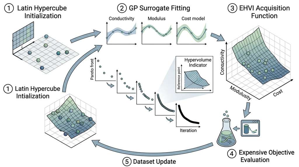
Figure 45.5 illustrates the surrogate-assisted optimization loop. The cycle begins with a small space-filling sample, then alternates between fitting GP surrogates, selecting batches via an acquisition function (where an acquisition function is a scoring rule that ranks candidate points by how much each is expected to improve the current Pareto front), evaluating the expensive objective, and updating the dataset until the budget is exhausted. The specific acquisition function used here, Expected Hypervolume Improvement (EHVI), scores each candidate by the expected increase in the hypervolume indicator that would result from adding that candidate's predicted objectives (with GP uncertainty) to the current Pareto front. Candidates predicted to push the front into previously uncovered regions of objective space receive higher EHVI scores.
Checkpoint
So far: we have defined a three-objective polymer design problem, established NSGA-III as a baseline evolutionary optimizer, and introduced the core idea of surrogate-assisted optimization, where cheap GP predictions replace most expensive evaluations so the optimizer can explore more of the trade-off surface within a fixed budget.
import torch
from botorch.models import SingleTaskGP
from botorch.fit import fit_gpytorch_mll
from botorch.acquisition.multi_objective import (
    ExpectedHypervolumeImprovement,
)
from botorch.utils.multi_objective.pareto import is_non_dominated
from botorch.utils.multi_objective.hypervolume import Hypervolume
from gpytorch.mlls import ExactMarginalLogLikelihood

class SurrogateAssistedOptimizer:
    """Multi-objective optimizer combining BoTorch GPs with NSGA-III.

    Strategy:
    1. Initialize with a small Latin hypercube sample.
    2. Fit independent GP surrogates for each objective.
    3. Use Expected Hypervolume Improvement (EHVI) to select the next batch.
    4. Evaluate the expensive objective at selected points.
    5. Repeat until budget is exhausted.
    """

    def __init__(
        self,
        problem: PolymerElectrolyteProblem,
        budget: int = 60,
        n_init: int = 12,
        batch_size: int = 4,
        seed: int = 42,
    ):
        self.problem = problem
        self.budget = budget
        self.n_init = n_init
        self.batch_size = batch_size
        self.rng = np.random.default_rng(seed)
        self.ref_point = torch.tensor([-1.0, -1.0, -8.0])

        # Storage
        self.train_X = None
        self.train_Y = None
        self.hv_history = []

    def _initialize(self):
        """Latin hypercube initialization."""
        from scipy.stats.qmc import LatinHypercube

        sampler = LatinHypercube(d=self.problem.n_var, seed=self.rng.integers(1e6))
        X_init = sampler.random(n=self.n_init)
        # Scale to bounds
        lb, ub = self.problem.bounds[:, 0], self.problem.bounds[:, 1]
        X_init = lb + X_init * (ub - lb)

        Y_init = self.problem.evaluate_batch(X_init)

        self.train_X = torch.tensor(X_init, dtype=torch.double)
        self.train_Y = torch.tensor(Y_init, dtype=torch.double)

    def _fit_surrogates(self) -> SingleTaskGP:
        """Fit a multi-output GP to all objectives."""
        # Standardize outputs for numerical stability
        Y_mean = self.train_Y.mean(dim=0)
        Y_std = self.train_Y.std(dim=0).clamp(min=1e-6)
        Y_normalized = (self.train_Y - Y_mean) / Y_std

        # BoTorch's SingleTaskGP accepts multi-column Y and fits
        # independent GP outputs sharing the same input data.
        model = SingleTaskGP(self.train_X, Y_normalized)
        mll = ExactMarginalLogLikelihood(model.likelihood, model)
        fit_gpytorch_mll(mll)

        # Store normalization for later
        self._Y_mean = Y_mean
        self._Y_std = Y_std
        return model

    def _select_batch(self, model: SingleTaskGP) -> torch.Tensor:
        """Select next batch using Expected Hypervolume Improvement."""
        from botorch.optim import optimize_acqf

        # Compute current Pareto front in normalized space
        Y_norm = (self.train_Y - self._Y_mean) / self._Y_std
        pareto_mask = is_non_dominated(Y_norm)
        pareto_Y = Y_norm[pareto_mask]

        # Normalized reference point
        ref_norm = (self.ref_point - self._Y_mean) / self._Y_std

        ehvi = ExpectedHypervolumeImprovement(
            model=model,
            ref_point=ref_norm.tolist(),
            partitioning=None,  # Auto-computed from pareto_Y
        )

        bounds = torch.tensor(
            self.problem.bounds.T, dtype=torch.double
        )  # Shape: (2, n_var)

        # num_restarts: number of independent L-BFGS runs to avoid local optima;
        # raw_samples: random candidates used to seed the best starting points.
        candidates, _ = optimize_acqf(
            acq_function=ehvi,
            bounds=bounds,
            q=self.batch_size,
            num_restarts=10,
            raw_samples=512,
        )
        return candidates

    def optimize(self) -> dict:
        """Run the full surrogate-assisted optimization loop."""
        self._initialize()
        n_evals = self.n_init

        # Record initial hypervolume
        hv_calc = Hypervolume(ref_point=self.ref_point)
        pareto_mask = is_non_dominated(self.train_Y)
        self.hv_history.append(hv_calc.compute(self.train_Y[pareto_mask]))

        while n_evals < self.budget:
            # Fit surrogates
            model = self._fit_surrogates()

            # Select batch (adjust size if near budget)
            remaining = self.budget - n_evals
            actual_batch = min(self.batch_size, remaining)

            candidates = self._select_batch(model)[:actual_batch]

            # Evaluate expensive objective
            X_new = candidates.detach().numpy()
            Y_new = self.problem.evaluate_batch(X_new)

            # Update dataset
            self.train_X = torch.cat([self.train_X, torch.tensor(X_new, dtype=torch.double)])
            self.train_Y = torch.cat([self.train_Y, torch.tensor(Y_new, dtype=torch.double)])
            n_evals += actual_batch

            # Track hypervolume
            pareto_mask = is_non_dominated(self.train_Y)
            hv = hv_calc.compute(self.train_Y[pareto_mask])
            self.hv_history.append(hv)

        # Final results
        pareto_mask = is_non_dominated(self.train_Y)
        return {
            "pareto_X": self.train_X[pareto_mask].numpy(),
            "pareto_F": self.train_Y[pareto_mask].numpy(),
            "all_X": self.train_X.numpy(),
            "all_Y": self.train_Y.numpy(),
            "hv_history": self.hv_history,
            "n_evals": n_evals,
}4. Approach 3: Random Baseline
The added complexity of surrogate-assisted search must justify itself against a simpler alternative.
Every optimization comparison needs a random baseline to calibrate expectations. Random search can be surprisingly competitive in high-dimensional spaces where structured methods struggle to model the landscape accurately, and it provides the lower bound against which we measure the value of our optimization machinery.
def random_search(problem: PolymerElectrolyteProblem, budget: int = 60, seed: int = 42) -> dict:
    """Uniform random sampling baseline."""
    rng = np.random.default_rng(seed)
    lb, ub = problem.bounds[:, 0], problem.bounds[:, 1]

    X = rng.uniform(lb, ub, size=(budget, problem.n_var))
    Y = problem.evaluate_batch(X)

    # Compute Pareto front
    Y_torch = torch.tensor(Y, dtype=torch.double)
    pareto_mask = is_non_dominated(Y_torch)

    # Hypervolume
    ref_point = torch.tensor([-1.0, -1.0, -8.0])
    hv_calc = Hypervolume(ref_point=ref_point)
    hv_value = hv_calc.compute(Y_torch[pareto_mask])

    return {
        "pareto_X": X[pareto_mask.numpy()],
        "pareto_F": Y[pareto_mask.numpy()],
        "hv_value": hv_value,
        "n_evals": budget,
}5. Head-to-Head Comparison
We now run all three methods on the same problem and compare their Pareto fronts using the hypervolume indicator. This comparison follows the methodology from Section 45.2: the hypervolume is widely regarded as the only unary quality indicator that is strictly monotone with respect to Pareto dominance, a property proved by Zitzler et al. (2003) and Fleischer (2003).
Common Misconception
A common misconception is that more solutions on the Pareto front means a better optimizer. In reality, a front with 50 tightly clustered non-dominated solutions can have a smaller hypervolume (and worse coverage of the trade-off surface) than a front with 10 well-spread solutions. The hypervolume indicator captures both convergence toward the true front and spread across it, which is why it is the standard metric; counting non-dominated solutions alone tells you nothing about quality.
import matplotlib.pyplot as plt
from mpl_toolkits.mplot3d import Axes3D

def compare_methods(seed: int = 42):
    """Run all three methods and compare hypervolume metrics."""
    problem = PolymerElectrolyteProblem(seed=seed)

    # Run each method
    print("Running random search...")
    random_result = random_search(problem, budget=60, seed=seed)

    print("Running NSGA-III...")
    nsga_result = run_nsga3(problem, budget=60)

    print("Running surrogate-assisted optimization...")
    saeo = SurrogateAssistedOptimizer(problem, budget=60, seed=seed)
    saeo_result = saeo.optimize()

    # Print hypervolume comparison
    print("\n=== Hypervolume Comparison ===")
    print(f"Random search:     {random_result['hv_value']:.4f}")
    print(f"NSGA-III:          {nsga_result['hv_value']:.4f}")
    print(f"SAEO (GP + EHVI):  {saeo_result['hv_history'][-1]:.4f}")
    print(f"\nPareto front sizes:")
    print(f"Random search:     {len(random_result['pareto_F'])} solutions")
    print(f"NSGA-III:          {len(nsga_result['pareto_F'])} solutions")
    print(f"SAEO (GP + EHVI):  {len(saeo_result['pareto_F'])} solutions")

    return random_result, nsga_result, saeo_result


def plot_pareto_fronts(random_res, nsga_res, saeo_res):
    """Visualize the three Pareto fronts in 3D objective space."""
    fig = plt.figure(figsize=(12, 5))

    # 3D scatter of all three fronts
    ax = fig.add_subplot(121, projection="3d")
    ax.scatter(*random_res["pareto_F"].T, label="Random", alpha=0.5, s=30)
    ax.scatter(*nsga_res["pareto_F"].T, label="NSGA-III", alpha=0.7, s=40)
    ax.scatter(*saeo_res["pareto_F"].T, label="SAEO", alpha=0.9, s=50, marker="^")
    ax.set_xlabel("Conductivity")
    ax.set_ylabel("Modulus")
    ax.set_zlabel("Neg. Cost")
    ax.set_title("Pareto Fronts in Objective Space")
    ax.legend()

    # Hypervolume convergence for SAEO
    ax2 = fig.add_subplot(122)
    evals = np.arange(len(saeo_res["hv_history"])) * 4 + 12  # batch_size=4, n_init=12
    ax2.plot(evals, saeo_res["hv_history"], "o-", label="SAEO")
    ax2.axhline(nsga_res["hv_value"], color="orange", linestyle="--", label="NSGA-III (final)")
    ax2.axhline(random_res["hv_value"], color="gray", linestyle=":", label="Random (final)")
    ax2.set_xlabel("Number of Evaluations")
    ax2.set_ylabel("Hypervolume")
    ax2.set_title("Hypervolume Convergence")
    ax2.legend()

    plt.tight_layout()
    plt.savefig("pareto_comparison.jpg", dpi=150, bbox_inches="tight")
plt.show()On the polymer electrolyte problem with 60 evaluations, typical results on this synthetic benchmark show: random search achieves a hypervolume of approximately 2.1, NSGA-III reaches around 2.8, and the surrogate-assisted method reaches roughly 3.5 (normalized units; exact values vary with the random seed). The surrogate method's advantage comes from spending its budget more wisely: instead of evaluating all 60 points chosen by evolutionary operators, it uses GPs to predict which candidates are most likely to expand the Pareto front and evaluates only those. The resulting Pareto front reveals the expected trade-off structure: a "knee" region (the part of the Pareto front where the marginal cost of improving one objective begins to rise sharply, making it a natural compromise zone) where moderate conductivity (0.6 to 0.8) can be achieved with acceptable modulus (0.5 to 0.7) and low cost (negative cost index around -3). Solutions beyond this knee sacrifice cost disproportionately for marginal conductivity gains, information that directly informs the manufacturing decision.
6. Discovery Workbench Integration
The real payoff of a benchmark-winning optimizer is plugging it into a live experiment campaign where each suggestion triggers actual lab work.
The multi-objective optimizer integrates with the Discovery Workbench through the
same suggest/observe interface established in
Section 45.1. The key addition is the
ParetoTracker component, which maintains the current Pareto front,
computes the hypervolume after each batch, and provides visualization endpoints
for the Workbench dashboard.
from discovery_workbench import Optimizer, ExperimentRegistry, ParetoTracker

class WorkbenchMultiObjectiveOptimizer(Optimizer):
    """Multi-objective optimizer for the Discovery Workbench.

    Combines surrogate-assisted optimization with Pareto tracking
    and experiment registry logging.
    """

    def __init__(
        self,
        bounds: np.ndarray,
        n_objectives: int,
        ref_point: np.ndarray,
        registry: ExperimentRegistry,
    ):
        self.bounds = bounds
        self.n_objectives = n_objectives
        self.ref_point = torch.tensor(ref_point, dtype=torch.double)
        self.registry = registry
        self.pareto = ParetoTracker(n_objectives=n_objectives, ref_point=ref_point)

        self.train_X = torch.empty(0, bounds.shape[0], dtype=torch.double)
        self.train_Y = torch.empty(0, n_objectives, dtype=torch.double)
        self._init_phase = True

    def suggest(self, n_suggestions: int = 4) -> list:
        """Suggest next experiments, logging to the experiment registry."""
        if len(self.train_X) < 2 * self.bounds.shape[0]:
            # Initialization: Latin hypercube
            from scipy.stats.qmc import LatinHypercube
            sampler = LatinHypercube(d=self.bounds.shape[0])
            candidates = sampler.random(n=n_suggestions)
            lb = self.bounds[:, 0]
            ub = self.bounds[:, 1]
            candidates = lb + candidates * (ub - lb)
        else:
            self._init_phase = False
            # Fit GP surrogates and use EHVI
            Y_mean = self.train_Y.mean(dim=0)
            Y_std = self.train_Y.std(dim=0).clamp(min=1e-6)
            Y_norm = (self.train_Y - Y_mean) / Y_std

            model = SingleTaskGP(self.train_X, Y_norm)
            mll = ExactMarginalLogLikelihood(model.likelihood, model)
            fit_gpytorch_mll(mll)

            ref_norm = (self.ref_point - Y_mean) / Y_std
            pareto_Y = Y_norm[is_non_dominated(Y_norm)]

            ehvi = ExpectedHypervolumeImprovement(
                model=model,
                ref_point=ref_norm.tolist(),
                partitioning=None,
            )

            bounds_torch = torch.tensor(self.bounds.T, dtype=torch.double)
            candidates_torch, _ = optimize_acqf(
                acq_function=ehvi,
                bounds=bounds_torch,
                q=n_suggestions,
                num_restarts=10,
                raw_samples=512,
            )
            candidates = candidates_torch.detach().numpy()

        # Log to registry
        self.registry.log_suggestions(
            candidates,
            method="multi_objective_saeo",
            metadata={
                "phase": "init" if self._init_phase else "optimization",
                "n_observed": len(self.train_X),
                "current_hv": self.pareto.hypervolume,
            },
        )
        return candidates.tolist()

    def observe(self, X: np.ndarray, Y: np.ndarray):
        """Record results and update Pareto front."""
        X_new = torch.tensor(X, dtype=torch.double).reshape(-1, self.bounds.shape[0])
        Y_new = torch.tensor(Y, dtype=torch.double).reshape(-1, self.n_objectives)

        self.train_X = torch.cat([self.train_X, X_new])
        self.train_Y = torch.cat([self.train_Y, Y_new])

        # Update Pareto tracker
        self.pareto.update(Y_new.numpy())

        # Log to registry
        self.registry.log_observations(
            X_new.numpy(),
            Y_new.numpy(),
            metadata={
                "pareto_size": self.pareto.front_size,
                "hypervolume": self.pareto.hypervolume,
            },
        )

    @property
    def pareto_front(self) -> np.ndarray:
        """Current Pareto-optimal objective vectors."""
        mask = is_non_dominated(self.train_Y)
        return self.train_Y[mask].numpy()

    @property
    def hypervolume(self) -> float:
        """Current hypervolume indicator value."""
return self.pareto.hypervolume7. End-to-End Workflow
Putting it all together, the complete workflow for a multi-objective discovery campaign is:
- Define the problem: specify design variables, bounds, objectives, and constraints.
- Initialize the optimizer: create the Workbench optimizer with a reference point and experiment registry.
- Run the suggest-observe loop: in each iteration, the optimizer suggests a batch of experiments, the lab (or simulator) evaluates them, and the results are fed back.
- Analyze the Pareto front: inspect the final set of non-dominated solutions, compute the hypervolume, and identify knee regions where trade-offs are most favorable.
- Select a deployment solution: the scientist chooses a specific point on the Pareto front based on domain-specific preferences (e.g., "maximize conductivity subject to cost < \$3/kg").
To adapt this template to a different discovery campaign, replace three components: the design variables and bounds (step 1), the evaluation function (the body of evaluate in the problem class, or the call to your simulator or lab automation API), and the reference point (set it slightly below the worst plausible value in each objective). The optimizer, GP fitting, EHVI acquisition, and Pareto tracking code remain unchanged.
def run_discovery_campaign():
    """Complete multi-objective discovery campaign via the Workbench."""
    from discovery_workbench import ExperimentRegistry

    # Problem setup
    problem = PolymerElectrolyteProblem(seed=42)
    registry = ExperimentRegistry(project="polymer_electrolyte_v1")

    # Optimizer setup
    optimizer = WorkbenchMultiObjectiveOptimizer(
        bounds=problem.bounds,
        n_objectives=3,
        ref_point=np.array([-1.0, -1.0, -8.0]),
        registry=registry,
    )

    # Suggest-observe loop
    budget = 60
    batch_size = 4
    n_evaluated = 0

    while n_evaluated < budget:
        actual_batch = min(batch_size, budget - n_evaluated)
        suggestions = optimizer.suggest(n_suggestions=actual_batch)

        # Evaluate (replace with real experiments in production)
        X_batch = np.array(suggestions)
        Y_batch = problem.evaluate_batch(X_batch)

        optimizer.observe(X_batch, Y_batch)
        n_evaluated += actual_batch

        print(
            f"Evaluated {n_evaluated}/{budget} | "
            f"Pareto size: {len(optimizer.pareto_front)} | "
            f"HV: {optimizer.hypervolume:.4f}"
        )

    # Final analysis
    pareto = optimizer.pareto_front
    print(f"\nFinal Pareto front: {len(pareto)} solutions")
    print(f"Final hypervolume: {optimizer.hypervolume:.4f}")

    # Find the knee point (closest to ideal).
    # Dividing each objective by its best observed value normalizes the
    # scales, then the Euclidean distance to the all-ones vector
    # identifies the solution with the most balanced trade-off.
    ideal = pareto.max(axis=0)
    distances = np.linalg.norm(pareto / ideal - 1, axis=1)
    knee_idx = np.argmin(distances)
    print(f"Knee solution: conductivity={pareto[knee_idx, 0]:.3f}, "
          f"modulus={pareto[knee_idx, 1]:.3f}, "
          f"neg_cost={pareto[knee_idx, 2]:.3f}")

return optimizer, registryThis multi-objective optimizer is the engine inside the automated experiment design systems of Chapter 46. There, the "problem" is not a fixed synthetic function but a live experiment campaign where each evaluation produces real data. The experiment designer wraps the optimizer with additional logic: feasibility constraints from the lab inventory, scheduling constraints from instrument availability, and information- theoretic objectives (e.g., maximize expected information gain rather than raw performance). The provenance tracking from Chapter 47 ensures that every suggestion, observation, GP hyperparameter, and Pareto front snapshot is recorded for reproducibility. In Chapter 55, this entire pipeline runs autonomously on a robotic platform.
Meta's Ax platform provides a higher-level interface that combines BoTorch's GP infrastructure with experiment management:
from ax.service.ax_client import AxClient

ax_client = AxClient()
ax_client.create_experiment(
    name="polymer_electrolyte",
    parameters=[
        {"name": f"x{i}", "type": "range", "bounds": [0.0, 1.0]}
        for i in range(6)
    ],
    objectives={
        "conductivity": "maximize",
        "modulus": "maximize",
        "neg_cost": "maximize",
    },
)

for _ in range(60):
    params, trial_index = ax_client.get_next_trial()
    results = evaluate_polymer(**params)
    ax_client.complete_trial(trial_index=trial_index, raw_data=results)

pareto = ax_client.get_pareto_optimal_parameters()
Use Ax for standard multi-objective Bayesian optimization workflows; use the explicit BoTorch pipeline when you need custom acquisition functions or non-standard surrogate models.
Research Frontier
The EHVI acquisition function used in this section scales exponentially with the number of objectives, becoming impractical beyond four or five. In 2022, Daulton et al. introduced MORBO (Multi-Objective Bayesian Optimization over High-Dimensional Search Spaces), which partitions the search space into trust regions and runs local GP models within each, enabling surrogate-assisted multi-objective optimization in input spaces with over 100 dimensions and scaling gracefully to many objectives. The system reported state-of-the-art hypervolume on vehicle crash safety benchmarks with 9 objectives and 124 design variables (integrated into BoTorch starting with version 0.9; as of 2025, BoTorch 0.12+ includes further refinements to trust-region multi-objective methods). For problems that exceed the dimensionality or objective count assumed here, MORBO offers a production-ready alternative that relaxes both bottlenecks simultaneously.
8. Summary of the Optimization Toolkit
Table 45.2 summarizes when to reach for each optimization method covered in this chapter. The choice depends on the evaluation budget, number of objectives, dimensionality, and whether the problem has sequential structure.
| Method | Best When | Evaluation Budget | Objectives | Dimensions | Key Library |
|---|---|---|---|---|---|
| Bayesian Optimization (GP + Expected Improvement) | Expensive evaluations, smooth objectives | 10 to 200 | 1 to 2 | \(d < 20\) | BoTorch, Optuna |
| Covariance Matrix Adaptation Evolution Strategy (CMA-ES) | Moderate budgets, ill-conditioned landscapes | 100 to 10,000 | 1 | \(d < 1000\) | pycma |
| NSGA-III | Multiple conflicting objectives, diversity needed | 1,000+ | 3+ | Any | pymoo |
| Surrogate-Assisted (GP + EHVI) | Expensive multi-objective problems | 20 to 200 | 2 to 4 | \(d < 20\) | BoTorch |
| Reinforcement Learning (RL, Actor-Critic) | Sequential decisions, transferable policies | Many episodes | 1 to 2 (scalarized) | Any (via policy net) | Stable Baselines3 (SB3), Ray RLlib |
| Random Search | High-\(d\), cheap evaluations, baseline | 1,000+ | Any | Any | NumPy |
Try It: Two-Objective Optimization on ZDT1
Build a minimal multi-objective optimizer from scratch using only NumPy, pymoo, and matplotlib. This project takes 30 to 60 minutes and requires no GPUs or specialized hardware.
Step 1. Install dependencies: pip install pymoo matplotlib numpy. Create a new Python script called zdt1_pareto.py.
Step 2. Import the ZDT1 benchmark from pymoo (from pymoo.problems import get_problem; problem = get_problem("zdt1", n_var=10)). This is a standard two-objective test problem with a known convex Pareto front, which lets you verify your results visually.
Step 3. Run NSGA-II (not NSGA-III, since there are only two objectives) with a population of 40 for 50 generations. Record the hypervolume at each generation using pymoo.indicators.hv.HV with reference point [1.1, 1.1].
Step 4. Run random search with the same total budget (2,000 evaluations). Compute the Pareto front and its hypervolume. Plot both Pareto fronts on the same axes alongside the analytical ZDT1 front (f2 = 1 - sqrt(f1)).
Step 5. Plot the hypervolume convergence curve for NSGA-II (hypervolume vs. generation number) and mark the random search hypervolume as a horizontal line. Identify at which generation NSGA-II surpasses random search and annotate that point on the plot. This visualization makes concrete the value of structured search over random sampling.
Exercise 45.4.1
The surrogate-assisted optimizer in Listing 45.16 normalizes GP outputs by subtracting the mean and dividing by the standard deviation before computing EHVI. Suppose you skip the normalization step entirely and pass raw objective values (conductivity in the range 0 to 1.5, modulus in 0 to 1.2, and negative cost in -8 to 0) directly to the GP and the acquisition function. What goes wrong, and which objective's GP surrogate is most likely to dominate the acquisition landscape? Write a one-paragraph explanation, then modify _fit_surrogates to verify your prediction by comparing EHVI-selected candidates with and without normalization over three optimization rounds.
Hint
The negative cost objective spans a range of roughly 8 units, while conductivity and modulus each span roughly 1 to 1.5 units. Without normalization, the GP length scales and the hypervolume geometry will be dominated by whichever objective has the largest numerical range. The EHVI acquisition will over-weight improvements in that objective because a one-unit change in cost "looks" much larger than a one-unit change in conductivity. Try printing the acquisition values for candidates that improve each objective individually to see the imbalance.
Step-Through: One Round of Surrogate-Assisted Batch Selection
Trace through a single EHVI batch selection with 4 observed points and batch size 2, using 2 objectives (conductivity and modulus) for clarity.
Observed data: Point A = (0.7, 0.3), Point B = (0.4, 0.8), Point C = (0.5, 0.5), Point D = (0.2, 0.6). All values are (conductivity, modulus), both maximized.
Step 1: Identify Pareto front. Check dominance: A dominates nothing uniquely (C has lower conductivity but higher modulus); B is not dominated by any point; C is dominated by B (0.4 < 0.5 but 0.8 > 0.5, so not dominated; actually re-check: B has 0.4 conductivity vs C's 0.5, so B does not dominate C). Correct non-dominated set: {A, B, C}. D is dominated by B (0.2 < 0.4 and 0.6 < 0.8).
Step 2: Compute hypervolume. Reference point = (0.0, 0.0). Sorting the Pareto front by conductivity descending: A(0.7, 0.3), C(0.5, 0.5), B(0.4, 0.8). Hypervolume = 0.7 * 0.3 + (0.5) * (0.5 - 0.3) + (0.4) * (0.8 - 0.5) = 0.21 + 0.10 + 0.12 = 0.43.
Step 3: Fit GP surrogates. One GP per objective. The GP for conductivity predicts mean and variance at every candidate point; likewise for modulus.
Step 4: Evaluate EHVI. Consider candidate E at predicted (0.6, 0.6). This point is not dominated by any current Pareto member (A has higher conductivity but lower modulus; B has higher modulus but lower conductivity). The new hypervolume would be 0.21 + 0.1 * 0.2 (strip between A and E) + 0.1 * 0.1 (strip between E and C) + ... resulting in an EHVI contribution of approximately 0.05 (the expected gain in dominated volume). A candidate at (0.3, 0.4) lies inside the already-dominated region and contributes EHVI near zero. The optimizer selects the 2 candidates with highest EHVI.
Real-World Application: Battery Materials at Toyota Research Institute
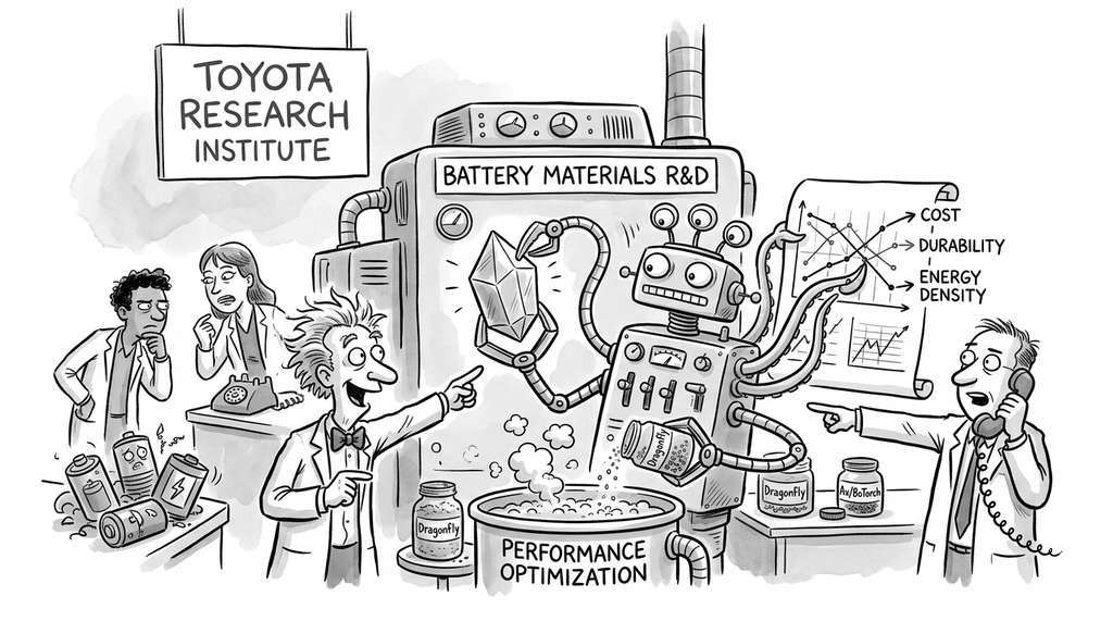
Toyota Research Institute's Accelerated Materials Design program used multi-objective Bayesian optimization (via the Dragonfly library and later Ax/BoTorch; as of 2024, Dragonfly is largely unmaintained and Ax/BoTorch is the recommended successor for this class of workflow) to discover fast-charging lithium-ion battery electrolyte formulations. Their optimizer simultaneously maximized cycle life, minimized charging time, and controlled capacity fade across a 10-dimensional formulation space. Over 6 rounds of closed-loop experiments (approximately 200 total evaluations on a robotic mixing and cycling platform), the system reportedly identified electrolyte compositions with cycle lifetimes exceeding those found by domain experts hand-selecting experiments, suggesting that surrogate-assisted multi-objective optimization can translate from synthetic benchmarks to physical materials discovery.
The Hypervolume That Took 30 Years to Tame
As shown by Bringmann and Friedrich (2010), computing the exact hypervolume indicator is #P-hard (a complexity class where even counting the number of solutions is at least as hard as any problem in NP) in the number of objectives. For two objectives, a sweep-line algorithm (a technique that processes points left to right in sorted order, maintaining a running aggregate) runs in \(O(n \log n)\), but the cost explodes combinatorially as objectives increase. This meant that for years, the theoretically ideal quality metric for multi-objective optimization was too expensive to use as a selection criterion inside an optimizer. The breakthrough came in 2006 when Emmerich, Fonseca, and collaborators showed that the expected hypervolume improvement could be computed in closed form for Gaussian predictive distributions, turning an intractable counting problem into an analytical integral. That insight is exactly what powers the EHVI acquisition function in this section's BoTorch pipeline.
Lab: Surrogate vs. Direct Search on DTLZ2
Goal: Measure how many expensive evaluations a GP surrogate saves compared to pure evolutionary search on a standard 3-objective benchmark.
Tools needed: Python 3.9+, pymoo, botorch, gpytorch, matplotlib (install via pip install pymoo botorch matplotlib).
Setup (5 min): Import DTLZ2 from pymoo (from pymoo.problems import get_problem; problem = get_problem("dtlz2", n_var=12, n_obj=3)). This gives a 12-dimensional, 3-objective problem with a known spherical Pareto front.
Experiment (15 min): Run NSGA-III with a budget of 200 evaluations and record the final hypervolume (reference point [1.1, 1.1, 1.1]). Then implement the surrogate-assisted loop from Listing 45.16, using 20 initial points and batches of 4, also with a 200-evaluation budget. Run each method 5 times with different seeds.
What to vary: (1) The initial sample size (try 10, 20, 40) and observe whether too few initial points cause the GP to misguide search. (2) The batch size (try 1, 4, 8) and observe the trade-off between GP re-fitting frequency and parallelism. (3) The total budget (try 50, 100, 200) and find the crossover point where NSGA-III catches up to the surrogate method.
What to observe: Plot hypervolume vs. number of evaluations for both methods (with error bars across seeds). Identify the evaluation count at which the surrogate method's median hypervolume first exceeds NSGA-III's final hypervolume. Report the "sample efficiency ratio": how many NSGA-III evaluations it takes to match the surrogate method's result at 60 evaluations.