32.4 Building a Bayesian Discovery Model

1. The Scientific Scenario: Enzyme Kinetics

A single S-shaped curve in an enzyme assay can upend decades of assumed kinetics: does the protein cooperate with itself during substrate binding, or is the sigmoid just measurement noise? A biochemistry lab is investigating exactly this question, studying how an enzyme's reaction rate \(v\) depends on substrate concentration \([S]\), and two competing hypotheses are on the table:

Hypothesis 1: Michaelis-Menten kinetics. The enzyme follows the classic single-substrate model:

where \(V_{\max}\) is the maximum rate and \(K_m\) is the Michaelis constant (the substrate concentration at half-maximal rate). This model assumes a single binding site with no cooperativity.

Hypothesis 2: Hill kinetics. The enzyme exhibits cooperative binding, described by the Hill equation:

where \(n\) is the Hill coefficient. When \(n > 1\), the enzyme shows positive cooperativity (binding of one substrate molecule makes subsequent binding easier); when \(n < 1\), negative cooperativity; when \(n = 1\), the Hill equation reduces to Michaelis-Menten. Note that the Michaelis-Menten model is nested within the Hill model as a special case.

With the theoretical distinction between these two models clear, the next step is to confront them with actual measurements. The lab has collected 15 measurements at different substrate concentrations. The question: does the data support cooperativity, or is the simpler Michaelis-Menten model sufficient? In short: encode each competing hypothesis as a generative model, let the posterior score them, and let information gain point to the experiment that settles the question fastest.

import numpy as np
import pymc as pm
import arviz as az

# Experimental data: substrate concentrations and observed rates
# (realistic enzyme kinetics with mild positive cooperativity)
rng = np.random.default_rng(42)
substrate_conc = np.array([
    0.1, 0.2, 0.5, 1.0, 2.0, 3.0, 5.0, 7.0,
    10.0, 15.0, 20.0, 30.0, 50.0, 75.0, 100.0
])

# True parameters: Hill kinetics with n=1.4 (mild cooperativity)
true_vmax = 120.0   # nmol/min
true_k05 = 8.0      # uM
true_n = 1.4         # Hill coefficient
true_sigma = 5.0     # measurement noise (nmol/min)

# Generate observed rates
true_rate = true_vmax * substrate_conc**true_n / (true_k05**true_n + substrate_conc**true_n)
observed_rate = true_rate + rng.normal(0, true_sigma, len(substrate_conc))
observed_rate = np.maximum(observed_rate, 0.1)  # rates must be positive

2. Encoding Hypotheses as PyMC Models

Choosing the wrong kinetic model can cascade into flawed drug dosing, missed cooperativity in a therapeutic target, or months of wasted follow-up experiments chasing an artifact of model misspecification. The encoding step that follows is what prevents those failures.

Each hypothesis becomes a complete generative model, where a generative model is a probabilistic specification that can simulate synthetic datasets from its priors and likelihood, not just fit existing observations. The priors are informed by biochemical domain knowledge. The priors encode what a biochemist knows before seeing this particular dataset. \(V_{\max}\) is positive and typically in the range 1-1000 nmol/min for enzymes of this class. \(K_m\) and \(K_{0.5}\) are positive and typically 0.1-100 \(\mu\)M. The Hill coefficient is positive and rarely exceeds 4 in naturally occurring enzymes.

def build_michaelis_menten(substrate, rates):
    """Hypothesis 1: Standard Michaelis-Menten kinetics.

    v = V_max * [S] / (K_m + [S])
    """
    with pm.Model() as mm_model:
        # Priors informed by biochemical domain knowledge
        log_vmax = pm.Normal("log_vmax", mu=np.log(100), sigma=1.5)
        log_km = pm.Normal("log_km", mu=np.log(10), sigma=1.5)
        sigma = pm.HalfNormal("sigma", sigma=20)

        # Transform to natural scale
        vmax = pm.math.exp(log_vmax)
        km = pm.math.exp(log_km)

        # Michaelis-Menten rate equation
        mu = vmax * substrate / (km + substrate)

        # Likelihood: normal measurement noise
        pm.Normal("obs", mu=mu, sigma=sigma, observed=rates)

    return mm_model

def build_hill(substrate, rates):
    """Hypothesis 2: Hill kinetics with cooperativity.

    v = V_max * [S]^n / (K_0.5^n + [S]^n)
    """
    with pm.Model() as hill_model:
        # Same Vmax and K priors as Michaelis-Menten
        log_vmax = pm.Normal("log_vmax", mu=np.log(100), sigma=1.5)
        log_k05 = pm.Normal("log_k05", mu=np.log(10), sigma=1.5)

        # Hill coefficient prior: centered on 1 (no cooperativity),
        # weakly allowing values from ~0.3 to ~4
        n_hill = pm.TruncatedNormal("n_hill", mu=1.0, sigma=0.8, lower=0.1, upper=5.0)

        sigma = pm.HalfNormal("sigma", sigma=20)

        # Transform to natural scale
        vmax = pm.math.exp(log_vmax)
        k05 = pm.math.exp(log_k05)

        # Hill rate equation
        mu = vmax * substrate**n_hill / (k05**n_hill + substrate**n_hill)

        # Likelihood
        pm.Normal("obs", mu=mu, sigma=sigma, observed=rates)

    return hill_model

mm_model = build_michaelis_menten(substrate_conc, observed_rate)
hill_model = build_hill(substrate_conc, observed_rate)

3. Prior Predictive Checks

Both models are now fully specified, so the next safeguard confirms that the chosen priors generate scientifically plausible reaction rates before committing to expensive posterior sampling. This catches prior miscalibration before it contaminates the posterior.

A prior predictive check samples parameter values from your chosen priors, pushes those samples forward through the model's likelihood to generate simulated data, and never conditions on observations. It matters because priors that look reasonable in parameter space can produce absurd predictions in data space. A seemingly mild log-normal prior on \(V_{\max}\), for example, might generate reaction rates of a million nmol/min. The mechanism: draw \(\theta \sim p(\theta)\), compute \(y_{\text{sim}} \sim p(y \mid \theta)\), and check whether the distribution of \(y_{\text{sim}}\) covers the range of values you would consider physically possible. Run prior predictive checks whenever you specify a new model. Switch to sensitivity analysis or prior elicitation from domain experts when the prior predictive distribution is too wide or too narrow despite reasonable-looking parameter priors.

# Prior predictive checks for both models
with mm_model:
    mm_prior = pm.sample_prior_predictive(draws=500, random_seed=42)

with hill_model:
    hill_prior = pm.sample_prior_predictive(draws=500, random_seed=42)

# Check: do the prior predictive samples span a reasonable range?
mm_prior_obs = mm_prior.prior_predictive["obs"].values.flatten()
hill_prior_obs = hill_prior.prior_predictive["obs"].values.flatten()

print("Michaelis-Menten prior predictive range:")
print(f"  2.5th percentile: {np.percentile(mm_prior_obs, 2.5):.1f}")
print(f"  97.5th percentile: {np.percentile(mm_prior_obs, 97.5):.1f}")
print(f"  Fraction negative: {(mm_prior_obs < 0).mean():.3f}")

print("\nHill prior predictive range:")
print(f"  2.5th percentile: {np.percentile(hill_prior_obs, 2.5):.1f}")
print(f"  97.5th percentile: {np.percentile(hill_prior_obs, 97.5):.1f}")
print(f"  Fraction negative: {(hill_prior_obs < 0).mean():.3f}")

4. Posterior Inference With Full Diagnostics

We fit both models with NUTS and run the complete convergence diagnostic suite from Section 32.2. For a model comparison to be trustworthy, both models must have converged; comparing a well-fit model to a poorly-fit one is meaningless.

def fit_and_diagnose(model, model_name, draws=3000, tune=1500):
    """Fit a model with NUTS and return trace with full diagnostics."""
    with model:
        trace = pm.sample(
            draws=draws, tune=tune, chains=4,
            target_accept=0.95,
            random_seed=42,
        )
        # Posterior predictive for model comparison
        pm.sample_posterior_predictive(trace, extend_inferencedata=True)

    # Convergence diagnostics
    rhat_max = max(
        float(az.rhat(trace)[v].max()) for v in az.rhat(trace).data_vars
    )
    ess_min = min(
        float(az.ess(trace, method="bulk")[v].min())
        for v in az.ess(trace, method="bulk").data_vars
    )
    divs = int(trace.sample_stats["diverging"].sum().values)

    print(f"\n{'='*50}")
    print(f"Model: {model_name}")
    print(f"  R-hat max: {rhat_max:.4f} {'PASS' if rhat_max < 1.01 else 'FAIL'}")
    print(f"  ESS bulk min: {ess_min:.0f} {'PASS' if ess_min > 400 else 'FAIL'}")
    print(f"  Divergences: {divs} {'PASS' if divs == 0 else 'FAIL'}")
    print(f"{'='*50}")

    return trace

mm_trace = fit_and_diagnose(mm_model, "Michaelis-Menten")
hill_trace = fit_and_diagnose(hill_model, "Hill Kinetics")

# Posterior summaries
print("\nMichaelis-Menten posterior:")
print(az.summary(mm_trace, var_names=["log_vmax", "log_km", "sigma"], hdi_prob=0.94))

print("\nHill posterior:")
print(az.summary(hill_trace, var_names=["log_vmax", "log_k05", "n_hill", "sigma"],
                 hdi_prob=0.94))

5. Model Comparison With LOO-CV

With both posteriors in hand and convergence verified, we compare the models' predictive accuracy using LOO-CV. The comparison answers: which model better predicts held-out enzyme kinetics measurements?

# LOO-CV model comparison
comparison = az.compare(
    {"Michaelis-Menten": mm_trace, "Hill": hill_trace},
    ic="loo",
)
print("\nLOO-CV Model Comparison:")
print(comparison)

# Detailed pointwise diagnostics
loo_mm = az.loo(mm_trace, pointwise=True)
loo_hill = az.loo(hill_trace, pointwise=True)

print(f"\nMichaelis-Menten: {(loo_mm.pareto_k > 0.7).sum()} problematic observations")
print(f"Hill: {(loo_hill.pareto_k > 0.7).sum()} problematic observations")

# Pointwise elpd difference: where does Hill predict better?
elpd_diff = loo_hill.loo_i.values - loo_mm.loo_i.values
print(f"\nPointwise elpd difference (Hill - MM):")
print(f"  Mean: {elpd_diff.mean():.3f}")
print(f"  Observations where Hill is better: {(elpd_diff > 0).sum()}/{len(elpd_diff)}")

# Which substrate concentrations favor Hill?
better_at = substrate_conc[elpd_diff > 0]
print(f"  Substrate concentrations where Hill wins: {better_at}")

6. Expected Information Gain for the Next Experiment

The comparison reveals which model currently predicts better, but the lab wants to know: where should we measure next to most efficiently distinguish between the two hypotheses? Expected Information Gain (EIG) quantifies how much a new measurement at substrate concentration \(s^*\) would reduce our uncertainty about which model is correct, where the gain is measured as the expected shift in model posterior probabilities after observing the new data point.

The EIG at a candidate design point \(s^*\) is the expected Kullback-Leibler (KL) divergence (a measure of how much one probability distribution differs from another; larger values mean the new data point would shift our beliefs more) between the updated and current model posteriors:

In words, this formula says: for each possible outcome \(y^*\) we might observe at concentration \(s^*\), compute how much the model ranking would change, then average over all possible outcomes weighted by how likely each one is. A high EIG means the measurement would substantially shift our beliefs regardless of the outcome; a low EIG means both models predict similar results at that concentration, so measuring there would not help distinguish them.

We approximate this by forward-simulating measurements from both models and computing how each simulated outcome would shift the model comparison:

def expected_information_gain(
    mm_trace, hill_trace, candidate_concentrations, n_simulations=200
):
    """Compute expected information gain for each candidate concentration.

    Simulates new observations from each model's posterior predictive
    and measures how much the LOO-CV ranking would shift.

    Parameters
    ----------
    mm_trace, hill_trace : az.InferenceData
        Fitted traces for both models.
    candidate_concentrations : np.ndarray
        Substrate concentrations to evaluate.
    n_simulations : int
        Number of forward simulations per candidate.

    Returns
    -------
    eig : np.ndarray
        Expected information gain at each candidate concentration.
    """
    # Current model weights from LOO-CV
    current_comparison = az.compare(
        {"MM": mm_trace, "Hill": hill_trace}, ic="loo"
    )
    current_weights = current_comparison["weight"].values

    # Extract posterior samples for forward simulation
    mm_vmax = np.exp(mm_trace.posterior["log_vmax"].values.flatten())
    mm_km = np.exp(mm_trace.posterior["log_km"].values.flatten())
    mm_sigma = mm_trace.posterior["sigma"].values.flatten()

    hill_vmax = np.exp(hill_trace.posterior["log_vmax"].values.flatten())
    hill_k05 = np.exp(hill_trace.posterior["log_k05"].values.flatten())
    hill_n = hill_trace.posterior["n_hill"].values.flatten()
    hill_sigma = hill_trace.posterior["sigma"].values.flatten()

    rng = np.random.default_rng(42)
    eig = np.zeros(len(candidate_concentrations))

    for i, s_star in enumerate(candidate_concentrations):
        kl_divergences = []

        for _ in range(n_simulations):
            # Draw parameters from each posterior
            idx = rng.integers(len(mm_vmax))

            # Simulate observation under MM
            mm_pred = mm_vmax[idx] * s_star / (mm_km[idx] + s_star)
            y_mm = mm_pred + rng.normal(0, mm_sigma[idx])

            # Simulate observation under Hill
            hill_pred = (hill_vmax[idx] * s_star**hill_n[idx]
                        / (hill_k05[idx]**hill_n[idx] + s_star**hill_n[idx]))
            y_hill = hill_pred + rng.normal(0, hill_sigma[idx])

            # Compute log-likelihood ratio at the simulated points
            ll_mm_under_mm = -0.5 * ((y_mm - mm_pred) / mm_sigma[idx])**2
            ll_hill_under_mm = -0.5 * ((y_mm - hill_pred) / hill_sigma[idx])**2

            # Information gain approximation: absolute difference in log-likelihoods
            kl_divergences.append(abs(ll_mm_under_mm - ll_hill_under_mm))

        eig[i] = np.mean(kl_divergences)

    return eig

# Evaluate EIG across the concentration range
candidates = np.logspace(-1, 2, 50)  # 0.1 to 100 uM
eig = expected_information_gain(mm_trace, hill_trace, candidates)

# Find the optimal next experiment
best_idx = np.argmax(eig)
print(f"\nOptimal next measurement: [S] = {candidates[best_idx]:.2f} uM")
print(f"Expected information gain: {eig[best_idx]:.4f}")
print(f"This is where MM and Hill predictions diverge most.")

Mental Model

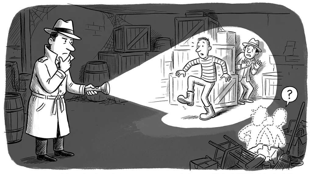
Think of Expected Information Gain like choosing where to shine a flashlight in a dark room to tell apart two suspects. If both suspects are standing in the same corner, shining the light there tells you nothing new: you see a figure either way. If they are both near the far wall, same problem. The flashlight is most useful aimed at the one spot where the suspects would be standing in different places, because only there does the beam distinguish one from the other. In enzyme kinetics, "shining the flashlight" means measuring at a substrate concentration, and the two suspects are the Michaelis-Menten and Hill models. EIG peaks at concentrations where the two models' predicted rates diverge most, just as the flashlight is most informative where the suspects' positions differ.

7. The Complete Discovery Pipeline

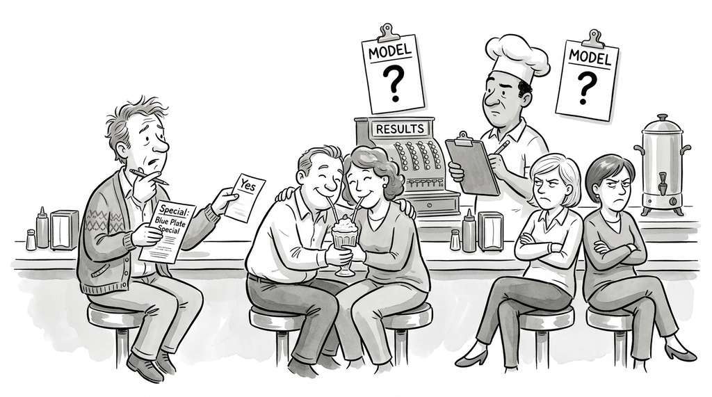
The following function integrates data generation, inference, comparison, and experiment design into a single reusable pipeline. Figure 32.6 illustrates the six-stage loop that this pipeline implements, showing how each stage feeds into the next and where the loop terminates. It takes competing hypotheses, data, and candidate experiments and returns the full Bayesian analysis:

class BayesianDiscoveryPipeline:
    """End-to-end Bayesian hypothesis comparison and experiment design.

    Integrates the Bayesian workflow (Section 32.1), NUTS inference
    (Section 32.2), LOO-CV comparison (Section 32.3), and EIG-based
    experiment design into a single reusable component.
    """

    def __init__(self, model_builders, model_names, data):
        """
        Parameters
        ----------
        model_builders : list of callable
            Functions that build PyMC models given data.
        model_names : list of str
            Human-readable names for each model.
        data : dict
            Data to pass to each model builder.
        """
        self.model_builders = model_builders
        self.model_names = model_names
        self.data = data
        self.models = {}
        self.traces = {}
        self.comparison = None

    def fit_all(self, draws=3000, tune=1500, target_accept=0.95):
        """Fit all models with NUTS and verify convergence."""
        for name, builder in zip(self.model_names, self.model_builders):
            model = builder(**self.data)
            with model:
                trace = pm.sample(
                    draws=draws, tune=tune, chains=4,
                    target_accept=target_accept, random_seed=42,
                )
                pm.sample_posterior_predictive(trace, extend_inferencedata=True)

            self.models[name] = model
            self.traces[name] = trace

            # Verify convergence
            rhat_max = max(
                float(az.rhat(trace)[v].max())
                for v in az.rhat(trace).data_vars
            )
            if rhat_max > 1.01:
                print(f"WARNING: {name} has R-hat = {rhat_max:.4f}. "
                      f"Do not trust this posterior.")

        return self

    def compare(self, ic="loo"):
        """Compare all fitted models using LOO-CV or WAIC."""
        self.comparison = az.compare(self.traces, ic=ic)
        return self.comparison

    def design_next(self, candidate_points, n_simulations=200):
        """Compute EIG across candidate design points and return the optimal next experiment.

        Parameters
        ----------
        candidate_points : np.ndarray
            Candidate input values (e.g., substrate concentrations) to evaluate.
        n_simulations : int
            Number of forward simulations per candidate point.

        Returns
        -------
        dict with keys 'best_point', 'eig_profile', and 'candidate_points'.
        """
        if len(self.traces) != 2:
            raise ValueError("design_next currently supports exactly two models.")

        names = list(self.traces.keys())
        eig = expected_information_gain(
            self.traces[names[0]], self.traces[names[1]],
            candidate_points, n_simulations=n_simulations,
        )
        best_idx = np.argmax(eig)
        return {
            "best_point": candidate_points[best_idx],
            "eig_profile": eig,
            "candidate_points": candidate_points,
        }

    def report(self):
        """Generate a human-readable discovery report."""
        if self.comparison is None:
            self.compare()

        best_model = self.comparison.index[0]
        elpd_diff = self.comparison["d_loo"].values[1]
        dse = self.comparison["dse"].values[1]
        ratio = abs(elpd_diff / dse) if dse > 0 else float("inf")

        report_lines = [
            "=" * 60,
            "BAYESIAN DISCOVERY REPORT",
            "=" * 60,
            f"Models compared: {', '.join(self.model_names)}",
            f"Best model: {best_model}",
            f"elpd difference: {elpd_diff:.2f} (SE: {dse:.2f})",
            f"Strength of evidence: {ratio:.1f} SE",
        ]

        if ratio < 2:
            report_lines.append("Verdict: Models are INDISTINGUISHABLE. "
                              "Collect more data or accept the simpler model.")
        elif ratio < 5:
            report_lines.append("Verdict: MODERATE evidence for the preferred model. "
                              "Consider targeted experiments.")
        else:
            report_lines.append("Verdict: STRONG evidence for the preferred model.")

        report_lines.append("=" * 60)
        return "\n".join(report_lines)

# Usage: the enzyme kinetics discovery pipeline
pipeline = BayesianDiscoveryPipeline(
    model_builders=[
        lambda substrate, rates: build_michaelis_menten(substrate, rates),
        lambda substrate, rates: build_hill(substrate, rates),
    ],
    model_names=["Michaelis-Menten", "Hill"],
    data={"substrate": substrate_conc, "rates": observed_rate},
)
pipeline.fit_all()
print(pipeline.report())

# Design the next experiment
design = pipeline.design_next(np.logspace(-1, 2, 50))
print(f"Optimal next measurement: [S] = {design['best_point']:.2f} uM")

8. Integration With the Discovery Workbench

The BayesianDiscoveryPipeline class is designed for direct integration with the Discovery Workbench introduced in Chapter 6. The pipeline's fit_all(), compare(), design_next(), and report() methods map to the Workbench's experiment-run-analyze cycle. The EIG computation from Listing 32.23 plugs into the Workbench's experiment design module, enabling a fully automated discovery loop:

1. Specify: define competing hypotheses as model builders.
2. Fit: run posterior inference on available data.
3. Compare: rank models by predictive accuracy.
4. Design: compute EIG to select the next experiment.
5. Acquire: collect new data at the optimal design point.
6. Repeat: return to step 2 with the expanded dataset.

This loop enacts the discovery cycle from Chapter 2 in Bayesian form. Each iteration either strengthens the leading hypothesis or exposes model inadequacy, triggering model revision (a new builder added to the pipeline). The loop terminates when Expected Value of Perfect Information (EVPI), where EVPI is the maximum amount the decision-maker would pay for a perfect oracle revealing the true model, drops below the cost of the next experiment (Section 32.3), meaning additional data would not shift the conclusion.