39.1 Gap Analysis and Analogical Transfer

1. The Geometry of What We Do Not Know

In 1986, a library scientist with no medical training predicted that fish oil could treat Raynaud's disease, a painful circulatory disorder. He did not run an experiment. Instead, he noticed that two literatures that never cited each other contained the missing halves of the same argument. Don Swanson's reasoning was deceptively simple. If literature A establishes that compound X affects process Y, and literature B establishes that process Y drives disease Z, the combined literature implies "compound X might treat disease Z," even though no single paper states it. Experimentalists later confirmed the prediction.

Swanson's insight was that scientific knowledge is fragmented across communities. The hypothesis was not hidden; it was distributed. Modern knowledge graphs make this kind of reasoning systematic. Instead of manually tracing chains across two literatures, we can analyze the full graph structure to find places where connections are conspicuously absent. In short: The most fertile ground for the next discovery is not where knowledge is absent, but where two dense bodies of knowledge almost touch and no one has built the bridge.

2. Structural Hole Detection in Knowledge Graphs

Drug repurposing candidates, materials with untested applications, and cross-field theoretical connections routinely hide in plain sight for years, stranded between research communities that never read each other's papers. A systematic method for locating these cross-community gaps turns serendipity into strategy.

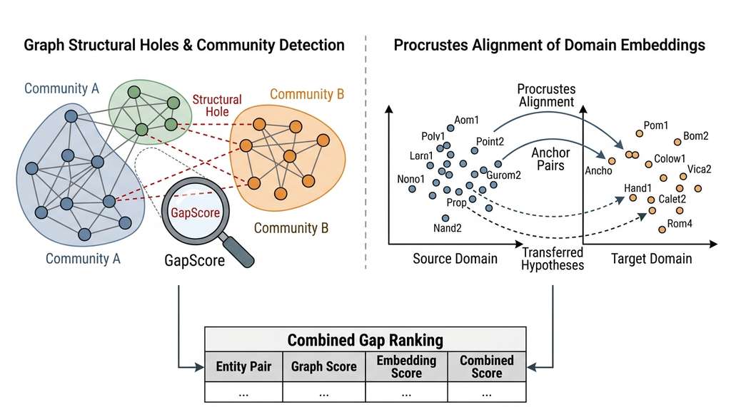
Ronald Burt's structural holes theory, originally from sociology, provides the conceptual framework. In a social network, a structural hole is a gap between two groups that are internally well-connected but have few bridges between them. Individuals who span structural holes gain access to diverse information and are disproportionately likely to generate good ideas. We apply the same logic to knowledge graphs: structural holes between well-studied subfields are prime locations for novel hypotheses. Figure 39.0 illustrates this core idea: two dense clusters of knowledge separated by a region with sparse or absent connections.

A structural hole is a position in a network where information flow between two dense clusters must pass through a few intermediary nodes, or has no path at all. The entities on either side represent separate pools of knowledge that no one has yet combined; connecting them often yields non-obvious insights. The detector scores every unconnected entity pair on three factors: how well-connected each entity is within its own neighborhood, how close the two entities sit via indirect paths, and how little their neighborhoods overlap. Use structural hole detection when you have a richly connected knowledge graph and want to prioritize cross-community hypotheses; for sparser graphs where topology alone is unreliable, prefer the embedding-space gap analysis described in Section 3.

Formalizing the Gap Score

Given a knowledge graph \(G = (V, E)\) where vertices are scientific entities (genes, proteins, compounds, diseases, phenomena) and edges are validated relations (interacts-with, causes, inhibits, co-occurs-with), we define a knowledge gap score for each pair of unconnected entities \((u, v) \notin E\):

where \(\mathcal{N}(u)\) is the neighborhood of \(u\), \(d(u, v)\) is the shortest-path distance, and the Jaccard complement (one minus the Jaccard similarity, measuring how little two sets overlap) term ensures we prioritize pairs with different neighborhoods (bridging distinct communities). High gap scores indicate entity pairs that are individually well-connected, relatively close in the graph, but occupy different neighborhoods: exactly the profile of a structural hole.

The following implementation uses NetworkX to compute gap scores across a biomedical knowledge graph:

import networkx as nx
import numpy as np
from itertools import combinations
from dataclasses import dataclass


@dataclass
class KnowledgeGap:
    """A scored gap in a knowledge graph."""
    entity_a: str
    entity_b: str
    gap_score: float
    shortest_path: int
    shared_neighbors: int
    community_a: int
    community_b: int


def detect_structural_holes(
    G: nx.Graph,
    max_distance: int = 4,
    min_degree: int = 3,
    top_k: int = 100,
) -> list[KnowledgeGap]:
    """Find structural holes in a knowledge graph.

    Identifies pairs of well-connected entities that lack a direct
    edge but occupy different graph communities, suggesting an
    undiscovered relation.

    Args:
        G: Knowledge graph (undirected for simplicity).
        max_distance: Maximum shortest-path distance to consider.
        min_degree: Minimum degree for candidate entities.
        top_k: Number of top-scoring gaps to return.
    """
    # Pre-compute communities using Louvain community detection,
    # a greedy modularity-optimization algorithm that partitions
    # graph nodes into densely connected groups
    communities = nx.community.louvain_communities(G, seed=42)
    node_to_community = {}
    for idx, comm in enumerate(communities):
        for node in comm:
            node_to_community[node] = idx

    # Filter to well-connected entities
    candidates = [n for n, d in G.degree() if d >= min_degree]

    # Pre-compute shortest paths (bounded)
    path_lengths = dict(
        nx.all_pairs_shortest_path_length(G, cutoff=max_distance)
    )

    gaps = []
    for u, v in combinations(candidates, 2):
        # Skip if edge already exists
        if G.has_edge(u, v):
            continue

        # Skip if too far apart or disconnected
        dist = path_lengths.get(u, {}).get(v)
        if dist is None or dist > max_distance:
            continue

        # Skip if in the same community (within-community gaps
        # are less likely to represent novel connections)
        comm_u = node_to_community[u]
        comm_v = node_to_community[v]
        if comm_u == comm_v:
            continue

        # Compute gap score
        neighbors_u = set(G.neighbors(u))
        neighbors_v = set(G.neighbors(v))
        intersection = neighbors_u & neighbors_v
        union = neighbors_u | neighbors_v

        jaccard_complement = 1.0 - len(intersection) / len(union)
        degree_product = len(neighbors_u) * len(neighbors_v)
        score = (degree_product / dist**2) * jaccard_complement

        gaps.append(KnowledgeGap(
            entity_a=u,
            entity_b=v,
            gap_score=score,
            shortest_path=dist,
            shared_neighbors=len(intersection),
            community_a=comm_u,
            community_b=comm_v,
        ))

    # Return top-k by gap score
    gaps.sort(key=lambda g: g.gap_score, reverse=True)
    return gaps[:top_k]

The following example applies this to a concrete biomedical knowledge graph. We construct a small but representative graph from drug-gene-disease relations and examine the top-scoring gaps:

# Build a sample biomedical knowledge graph
G = nx.Graph()

# Drug-gene interactions
drug_gene = [
    ("metformin", "AMPK"), ("metformin", "mTOR"),
    ("rapamycin", "mTOR"), ("rapamycin", "FKBP12"),
    ("aspirin", "COX2"), ("aspirin", "NFkB"),
    ("statins", "HMGCR"), ("statins", "NFkB"),
]

# Gene-disease associations
gene_disease = [
    ("AMPK", "type2_diabetes"), ("AMPK", "obesity"),
    ("mTOR", "cancer"), ("mTOR", "aging"),
    ("COX2", "inflammation"), ("COX2", "cancer"),
    ("NFkB", "inflammation"), ("NFkB", "autoimmune"),
    ("HMGCR", "cardiovascular"), ("FKBP12", "transplant_rejection"),
]

# Gene-gene interactions
gene_gene = [
    ("AMPK", "mTOR"), ("NFkB", "COX2"),
    ("AMPK", "NFkB"), ("mTOR", "FKBP12"),
]

G.add_edges_from(drug_gene + gene_disease + gene_gene)

# Detect structural holes
gaps = detect_structural_holes(G, min_degree=2, max_distance=4)
for gap in gaps[:5]:
    print(f"{gap.entity_a} <-> {gap.entity_b}: "
          f"score={gap.gap_score:.1f}, "
          f"path={gap.shortest_path}, "
          f"shared={gap.shared_neighbors}")

On a real knowledge graph with thousands of entities (built with techniques from Chapter 38), the detector typically surfaces hypotheses such as "metformin may affect aging through mTOR" and "statins may reduce inflammation through NFkB." Both are active research areas, suggesting that structural analysis of existing knowledge can in some cases independently recover connections that human researchers reach through years of incremental reasoning.

3. Embedding-Space Gap Analysis

Structural hole detection works on the discrete graph topology. But scientific knowledge also lives in continuous embedding spaces, where the distances between concepts encode semantic relationships. Tshitoyan et al. (2019) demonstrated this powerfully: word embeddings trained on materials science abstracts could predict future discoveries of thermoelectric materials years before those discoveries were published, simply by identifying materials whose embeddings were close to the concept "thermoelectric" but had never appeared in thermoelectric papers.

The geometric intuition is clean. In embedding space, well-studied relationships correspond to dense clusters of entity pairs. An embedding gap is a region of the space where the distance structure predicts a relationship, but no validated claim exists. Formally, given entity embeddings \(\mathbf{e}_u, \mathbf{e}_v \in \mathbb{R}^d\) and a relation embedding \(\mathbf{r} \in \mathbb{R}^d\), we look for triples \((u, r, v)\) where:

where \(\sigma\) is a scoring function (e.g., negative \(L_2\) distance or dot product), and \(\mathcal{K}\) is the set of known triples. This is precisely the link prediction formulation from Chapter 38, but reframed: instead of predicting missing links to complete a graph, we interpret high-scoring missing links as hypothesis candidates. In other words, a link predictor trained to fill in known gaps doubles as a hypothesis generator when pointed at unknown gaps, because the same embedding geometry that reconstructs validated relations also highlights where unvalidated relations are most plausible.

import numpy as np
from qdrant_client import QdrantClient
from qdrant_client.models import Distance, VectorParams, PointStruct


def find_embedding_gaps(
    entity_embeddings: dict[str, np.ndarray],
    known_pairs: set[tuple[str, str]],
    top_k: int = 50,
    distance_threshold: float = 0.3,
) -> list[tuple[str, str, float]]:
    """Find entity pairs that are close in embedding space
    but have no known relation.

    Uses Qdrant for efficient nearest-neighbor search over
    the entity embedding space.

    Args:
        entity_embeddings: Map from entity name to embedding vector.
        known_pairs: Set of (entity_a, entity_b) pairs with known relations.
        top_k: Number of gap candidates to return.
        distance_threshold: Maximum cosine distance to consider.
    """
    client = QdrantClient(":memory:")  # In-memory for demonstration
    dim = len(next(iter(entity_embeddings.values())))

    # Create collection and upload embeddings
    client.create_collection(
        collection_name="entities",
        vectors_config=VectorParams(size=dim, distance=Distance.COSINE),
    )

    points = [
        PointStruct(
            id=idx,
            vector=emb.tolist(),
            payload={"name": name},
        )
        for idx, (name, emb) in enumerate(entity_embeddings.items())
    ]
    client.upsert(collection_name="entities", points=points)

    # For each entity, find nearby entities without known relations
    gaps = []
    for name, emb in entity_embeddings.items():
        results = client.search(
            collection_name="entities",
            query_vector=emb.tolist(),
            limit=20,
        )
        for hit in results:
            other = hit.payload["name"]
            if other == name:
                continue
            pair = tuple(sorted([name, other]))
            if pair in known_pairs:
                continue
            distance = 1.0 - hit.score  # Convert similarity to distance
            if distance < distance_threshold:
                gaps.append((name, other, distance))

    # Deduplicate and sort by distance (closest = most interesting)
    seen = set()
    unique_gaps = []
    for a, b, dist in sorted(gaps, key=lambda x: x[2]):
        pair = tuple(sorted([a, b]))
        if pair not in seen:
            seen.add(pair)
            unique_gaps.append((a, b, dist))

    return unique_gaps[:top_k]

4. Analogical Transfer Across Domains

Gap analysis finds missing connections within a single knowledge structure. Analogical transfer finds missing connections between knowledge structures. The idea is ancient in science: Darwin drew on Malthus's population theory to develop natural selection. Rutherford modeled the atom on the solar system. Watson and Crick adapted the helical modeling approach from Linus Pauling's work on protein alpha-helix structure. In each case, a structural pattern from one domain was mapped onto another, generating a hypothesis that could not have arisen from within-domain reasoning alone.

Turning these celebrated historical examples into a repeatable method requires formalizing what "structural pattern" means and how to transfer it systematically.

Computationally, analogical transfer requires three steps: (1) identify structural patterns in a source domain, (2) find a mapping between source and target domain entities, and (3) project unmapped source relations onto the target domain as hypotheses. Gentner's Structure-Mapping Theory (SMT), where SMT is a cognitive science framework positing that analogies work by aligning relational structures rather than matching surface features, provides the theoretical framework: a good analogy preserves relational structure (the relations between entities) rather than surface features (the entities themselves). Gentner's key criterion, called systematicity, states that an analogy is stronger when it preserves an interconnected system of relations (such as a causal chain) rather than isolated pairings; the analogical transfer algorithm below operationalizes this by optimizing for a global alignment that preserves distances across all anchor pairs simultaneously, not just individual correspondences.

Mental Model

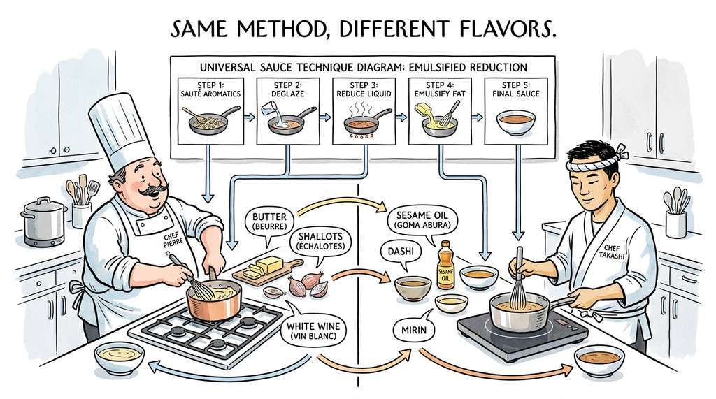
Think of analogical transfer as translating a recipe between cuisines. A French recipe for a particular sauce specifies ingredients (butter, shallots, white wine) and a structural pattern of operations (reduce a liquid with aromatics, then emulsify with fat). To "transfer" this recipe to Japanese cooking, you do not carry over the specific ingredients; you carry over the operational pattern and substitute local equivalents (mirin for wine, dashi for stock, sesame oil for butter). The anchor pairs are the known ingredient correspondences, and the Procrustes alignment (a mathematical technique for finding the best rotation to align two sets of points, defined formally below) is the mathematical equivalent of learning which French technique corresponds to which Japanese technique. A good culinary analogy preserves the why of each step (the structural relations) while swapping the what (the surface-level entities), and a bad analogy copies ingredients literally and produces something incoherent.

The "recipe translation" intuition translates directly into linear algebra.

We implement a simplified version using embedding alignment. If we have embeddings for entities in two domains, we learn a linear mapping \(\mathbf{W}\) that aligns the embedding spaces, then transfer relational patterns:

where \(\mathcal{A}\) is a set of anchor pairs (known analogies between domains), and the orthogonality regularizer preserves distances, preventing the mapping from collapsing the embedding structure. This is the same Procrustes alignment, a method that finds the orthogonal rotation matrix minimizing the sum of squared distances between paired point sets, used in cross-lingual word embedding alignment (Conneau et al., 2018), repurposed for cross-domain scientific analogy.

import numpy as np
from scipy.linalg import orthogonal_procrustes
from dataclasses import dataclass


@dataclass
class Analogy:
    """A cross-domain analogical hypothesis."""
    source_relation: tuple[str, str, str]  # (entity, relation, entity)
    target_hypothesis: tuple[str, str, str]
    confidence: float
    alignment_error: float


def learn_domain_alignment(
    source_embeddings: dict[str, np.ndarray],
    target_embeddings: dict[str, np.ndarray],
    anchor_pairs: list[tuple[str, str]],
) -> np.ndarray:
    """Learn a linear mapping between two domain embedding spaces.

    Uses orthogonal Procrustes alignment on anchor pairs (known
    cross-domain correspondences).

    Args:
        source_embeddings: Embeddings from the source domain.
        target_embeddings: Embeddings from the target domain.
        anchor_pairs: List of (source_entity, target_entity) pairs
            with known correspondences.

    Returns:
        Rotation matrix W that maps source to target space.
    """
    # Build aligned matrices from anchor pairs
    X = np.array([source_embeddings[s] for s, t in anchor_pairs])
    Y = np.array([target_embeddings[t] for s, t in anchor_pairs])

    # Orthogonal Procrustes: find W such that ||WX - Y|| is minimized
    # subject to W being orthogonal
    W, _ = orthogonal_procrustes(X, Y)
    return W


def transfer_hypotheses(
    source_relations: list[tuple[str, str, str]],
    source_embeddings: dict[str, np.ndarray],
    target_embeddings: dict[str, np.ndarray],
    W: np.ndarray,
    target_known_relations: set[tuple[str, str, str]],
    top_k: int = 20,
) -> list[Analogy]:
    """Transfer relational patterns from source to target domain.

    For each relation (a, r, b) in the source domain, maps a and b
    into the target embedding space and finds the nearest target
    entities to generate analogical hypotheses.

    Args:
        source_relations: Known relations in source domain.
        source_embeddings: Source domain entity embeddings.
        target_embeddings: Target domain entity embeddings.
        W: Alignment matrix from learn_domain_alignment.
        target_known_relations: Relations already known in target domain.
        top_k: Number of hypotheses to return.
    """
    target_names = list(target_embeddings.keys())
    target_matrix = np.array([target_embeddings[n] for n in target_names])

    analogies = []
    for src_a, rel, src_b in source_relations:
        # Map source entities into target space
        mapped_a = W @ source_embeddings[src_a]
        mapped_b = W @ source_embeddings[src_b]

        # Find nearest target entities
        dists_a = np.linalg.norm(target_matrix - mapped_a, axis=1)
        dists_b = np.linalg.norm(target_matrix - mapped_b, axis=1)

        tgt_a = target_names[np.argmin(dists_a)]
        tgt_b = target_names[np.argmin(dists_b)]

        # Skip if this relation is already known
        if (tgt_a, rel, tgt_b) in target_known_relations:
            continue

        # Confidence based on alignment quality
        err_a = float(np.min(dists_a))
        err_b = float(np.min(dists_b))
        confidence = 1.0 / (1.0 + err_a + err_b)

        analogies.append(Analogy(
            source_relation=(src_a, rel, src_b),
            target_hypothesis=(tgt_a, rel, tgt_b),
            confidence=confidence,
            alignment_error=err_a + err_b,
        ))

    analogies.sort(key=lambda a: a.confidence, reverse=True)
    return analogies[:top_k]

5. Combining Graph and Embedding Gaps

Structural hole detection and embedding-space gap analysis are complementary. Graph-based methods capture topological patterns (bridging positions, community boundaries) but miss semantic nuance. Embedding-based methods capture semantic similarity but miss structural context (how entities relate through intermediaries). The strongest hypothesis candidates appear in both analyses: entity pairs that bridge graph communities and are semantically close in embedding space.

We define a combined gap score that integrates both signals:

where \(\hat{G}\) and \(\hat{E}\) are min-max normalized (scaled linearly so that the smallest value maps to 0 and the largest maps to 1) versions of the structural gap score and the embedding proximity score (inverted distance), and \(\alpha\) controls the trade-off. In practice, \(\alpha = 0.5\) is a reasonable starting point, since it weights both signals equally before domain-specific tuning; domains with rich graph structure (biomedicine, chemistry) tend to benefit from higher \(\alpha\), while domains with sparser graphs but strong embeddings (materials science, social science) tend to benefit from lower \(\alpha\). Figure 39.1.1 illustrates structural hole detection and analogical transfer pipeline.

def combine_gap_signals(
    graph_gaps: list[KnowledgeGap],
    embedding_gaps: list[tuple[str, str, float]],
    alpha: float = 0.5,
) -> list[tuple[str, str, float, float, float]]:
    """Combine structural and embedding gap scores.

    Returns entity pairs ranked by a weighted combination of
    graph-based and embedding-based gap evidence.
    """
    # Normalize graph scores
    graph_dict = {
        (g.entity_a, g.entity_b): g.gap_score for g in graph_gaps
    }
    if graph_dict:
        g_min = min(graph_dict.values())
        g_max = max(graph_dict.values())
        g_range = g_max - g_min if g_max > g_min else 1.0
        graph_norm = {
            k: (v - g_min) / g_range for k, v in graph_dict.items()
        }
    else:
        graph_norm = {}

    # Normalize embedding scores (invert distance so higher = better)
    emb_dict = {
        tuple(sorted([a, b])): 1.0 - dist
        for a, b, dist in embedding_gaps
    }
    if emb_dict:
        e_min = min(emb_dict.values())
        e_max = max(emb_dict.values())
        e_range = e_max - e_min if e_max > e_min else 1.0
        emb_norm = {
            k: (v - e_min) / e_range for k, v in emb_dict.items()
        }
    else:
        emb_norm = {}

    # Combine: pairs appearing in both get the full combined score;
    # pairs in only one get a partial score
    all_pairs = set(graph_norm.keys()) | set(emb_norm.keys())
    results = []
    for pair in all_pairs:
        g_score = graph_norm.get(pair, 0.0)
        e_score = emb_norm.get(pair, 0.0)
        combined = alpha * g_score + (1 - alpha) * e_score
        results.append((pair[0], pair[1], combined, g_score, e_score))

    results.sort(key=lambda x: x[2], reverse=True)
    return results

Exercises

1. (Conceptual) Swanson's fish oil/Raynaud's disease connection required traversing exactly two disjoint literatures. In a knowledge graph, this corresponds to a path of length 2 through an intermediate concept. Generalize: what kinds of hypotheses require paths of length 3 or longer? Give a concrete example of a scientific hypothesis that would require a three-hop reasoning chain, and explain why it would be harder for a human scientist to discover compared to a two-hop chain.
2. (Coding) Implement a version of the structural hole detector that incorporates temporal information: for each gap, estimate the "age" of surrounding knowledge (when were the neighboring edges first established?) and weight gaps in recently active regions higher than gaps in dormant subfields. Apply this to a knowledge graph constructed from PubMed abstracts using the literature mining techniques from Chapter 36.
3. (Analysis) The embedding alignment approach assumes that cross-domain analogies are well-approximated by a single linear mapping. Design an experiment to test this assumption: split known cross-domain analogies into training (anchor pairs) and test sets, measure alignment quality as a function of the number of anchor pairs, and compare linear (Procrustes) alignment with a non-linear multi-layer perceptron (MLP)-based alignment. Under what conditions does the linear assumption break down?