26.4 Building a Domain Embedding Model

"They fine-tuned me on a million abstracts, and now I finally understand the difference between 'expression' in molecular biology and 'expression' in mathematics. Context is everything."

A Sentence Embedding That Found Its Domain

1. Why General Models Fall Short

Search a biomedical database for "BRCA1 expression in breast tissue." A general-purpose embedding model will cheerfully rank a paper about artistic expression in cancer awareness campaigns among the top results. Both texts share the same surface tokens in the same vector neighborhood. The model learned language from Wikipedia and Reddit, not from the laboratory, and it cannot tell that one "expression" belongs to molecular biology while the other belongs to the humanities.

With this distinction between vocabulary and geometry in mind, we can define exactly what a domain embedding model is and when it earns its place in a scientific pipeline.

In production scientific search systems, this mismatch between surface tokens and scientific meaning is not a minor inconvenience; it causes researchers to miss critical prior work, duplicate experiments that have already been published, and waste months pursuing directions the literature had already resolved. Building a domain embedding model is the direct fix for that failure mode.

What. Domain-specific embedding models are text encoders fine-tuned with contrastive objectives on scientific text, producing representations where semantic similarity reflects scientific relatedness rather than general linguistic similarity.

Why. Scientific retrieval, clustering, and classification require embeddings that capture domain-specific relationships. A general model might rank a genetics paper about "BRCA1 expression in breast tissue" as similar to a paper about "artistic expression in breast cancer awareness campaigns" because they share surface tokens. A domain model learns that the first paper relates to papers about tumor suppressors and DNA repair, not to papers about public health communication.

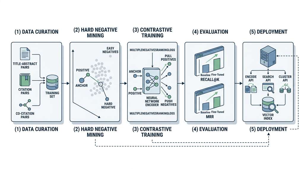
How. By fine-tuning a pretrained language model on pairs of related scientific texts (title-abstract, citation pairs, co-cited papers) using contrastive losses that pull related papers together and push unrelated ones apart. Figure 26.4.1 illustrates end-to-end domain embedding fine-tuning pipeline.

When. When your retrieval or clustering pipeline operates on scientific text and you observe that general embedding models conflate domain-specific terms, miss relevant papers, or produce clusters that do not align with scientific categories. In short: a domain embedding model teaches the vector space that scientific meaning is not the same as word overlap.

The full pipeline from raw scientific literature to a deployed domain embedding model follows five stages, illustrated in Figure 26.6. Each stage feeds into the next: curated training pairs supply the hard negative miner, which produces enriched triplets for contrastive fine-tuning, whose checkpoints are evaluated on domain benchmarks before the best model is deployed as the retrieval layer in the Discovery Workbench.

2. Data Curation: Building a Training Corpus

The quality of your domain embedding model depends critically on the quality of your training pairs. A pair of texts should be "positive" (semantically related) only if they share scientific meaning, not just surface tokens. The most reliable sources of scientific positive pairs are:

• Title-abstract pairs: A paper's title summarizes its abstract. This is a natural positive pair that captures the paper's core contribution. Available for millions of papers from Semantic Scholar, PubMed, and arXiv.
• Citation pairs: If paper A cites paper B, their abstracts are likely related. The citation context (the sentence in paper A that cites paper B) is an even stronger positive signal.
• Co-citation pairs: If papers A and B are frequently cited together by other papers, they address related topics.
• Same-MeSH-heading pairs: For biomedical text, papers sharing Medical Subject Headings (MeSH) terms address similar topics.

"""Data curation pipeline for scientific abstract training pairs."""
import json
import random
from dataclasses import dataclass
from pathlib import Path

@dataclass
class TrainingPair:
    """A positive pair for contrastive training."""
    anchor: str        # e.g., paper title or abstract
    positive: str      # e.g., related abstract
    source: str        # provenance: 'title-abstract', 'citation', etc.

def load_title_abstract_pairs(jsonl_path: str,
                               max_pairs: int = 100_000
                               ) -> list[TrainingPair]:
    """Load title-abstract pairs from a Semantic Scholar dump.

    Each line is: {"title": "...", "abstract": "...", "year": ...}
    Filters: non-empty title and abstract, English, after 2015.
    """
    pairs = []
    with open(jsonl_path, 'r', encoding='utf-8') as f:
        for line in f:
            if len(pairs) >= max_pairs:
                break
            record = json.loads(line)
            title = record.get('title', '').strip()
            abstract = record.get('abstract', '').strip()

            # Quality filters
            if not title or not abstract:
                continue
            if len(abstract.split()) < 50:  # skip very short abstracts
                continue
            if record.get('year', 0) < 2015:
                continue

            pairs.append(TrainingPair(
                anchor=title,
                positive=abstract,
                source='title-abstract'
            ))
    return pairs

def load_citation_pairs(citations_path: str,
                         abstracts: dict[str, str],
                         max_pairs: int = 100_000
                         ) -> list[TrainingPair]:
    """Build pairs from citation relationships.

    citations_path: JSONL with {"citing_id": ..., "cited_id": ...}
    abstracts: dict mapping paper_id -> abstract text
    """
    pairs = []
    with open(citations_path, 'r', encoding='utf-8') as f:
        for line in f:
            if len(pairs) >= max_pairs:
                break
            record = json.loads(line)
            citing = record['citing_id']
            cited = record['cited_id']

            if citing in abstracts and cited in abstracts:
                pairs.append(TrainingPair(
                    anchor=abstracts[citing],
                    positive=abstracts[cited],
                    source='citation'
                ))
    return pairs

def build_training_dataset(data_dir: str) -> list[TrainingPair]:
    """Combine multiple pair sources into a training set."""
    data_dir = Path(data_dir)

    # Load from multiple sources
    ta_pairs = load_title_abstract_pairs(
        str(data_dir / 'papers.jsonl'), max_pairs=200_000
    )
    print(f"Title-abstract pairs: {len(ta_pairs)}")

    # Combine and shuffle
    all_pairs = ta_pairs  # add citation pairs, etc.
    random.shuffle(all_pairs)

    print(f"Total training pairs: {len(all_pairs)}")
    print(f"Sources: { {s: sum(1 for p in all_pairs if p.source == s)
                        for s in set(p.source for p in all_pairs)} }")
    return all_pairs

3. Hard Negative Mining for Scientific Text

As covered in Section 26.2, hard negatives are critical for learning fine-grained distinctions. For scientific text, the most useful hard negatives are papers that share surface-level vocabulary but address different scientific questions. A paper about "CRISPR delivery in plant cells" and a paper about "CRISPR ethics in human gene therapy" share the term CRISPR but are scientifically distinct; they make an excellent hard negative pair.

Hard negative mining deliberately selects negative examples that the current model struggles to distinguish from true positives, rather than relying on random negatives. Random negatives (e.g., a Renaissance art paper paired against a molecular biology query) are easy to distinguish and provide almost zero gradient signal: the model already separates them, so it learns nothing. A pretrained embedding model finds corpus items whose embeddings fall close to the anchor but are not semantically related to the positive. The trainer then includes these "near-miss" items as explicit negatives. Use hard negative mining when your model plateaus with in-batch negatives (negatives drawn from other positive samples within the same training batch, rather than explicitly selected) alone, or when your domain contains many subfields that share vocabulary (e.g., "binding" in chemistry vs. immunology vs. computer science). For small, well-separated corpora where random negatives already yield strong gradients, in-batch negatives from MultipleNegativesRankingLoss may suffice without explicit mining.

Translating this principle into code requires a mining function that encodes the corpus, computes similarities against each anchor, and filters out items too close to the known positive.

The sentence-transformers library supports several negative mining strategies through its loss functions. The most effective for scientific text is the MultipleNegativesRankingLoss, which treats all other samples in the batch as negatives (like NT-Xent, where NT-Xent is the Normalized Temperature-scaled Cross-Entropy loss that treats every other item in the batch as a negative and scales similarities by a learned temperature), combined with explicit hard negative mining using a pretrained model to find near-misses.

"""Hard negative mining for scientific abstract pairs."""
import torch
import torch.nn.functional as F
import numpy as np
from sentence_transformers import SentenceTransformer

def mine_hard_negatives_for_abstracts(
    anchors: list[str],
    positives: list[str],
    corpus: list[str],
    model_name: str = 'all-MiniLM-L6-v2',
    n_negatives: int = 5,
    batch_size: int = 256
) -> list[list[str]]:
    """Mine hard negatives using a pretrained embedding model.

    For each anchor, find corpus items that are similar to the anchor
    but NOT in the positive set. These "near-miss" negatives provide
    the strongest training signal.

    Args:
        anchors: list of anchor texts (e.g., titles)
        positives: list of positive texts (e.g., abstracts)
        corpus: larger pool to mine negatives from
        model_name: pretrained model for initial similarity
        n_negatives: number of hard negatives per anchor
        batch_size: encoding batch size

    Returns:
        List of lists: hard negatives for each anchor
    """
    model = SentenceTransformer(model_name)

    # Encode anchors and corpus
    print("Encoding anchors...")
    anchor_embs = model.encode(
        anchors, batch_size=batch_size,
        show_progress_bar=True, convert_to_tensor=True
    )
    print("Encoding corpus...")
    corpus_embs = model.encode(
        corpus, batch_size=batch_size,
        show_progress_bar=True, convert_to_tensor=True
    )

    # Also encode positives to exclude them from negatives
    pos_embs = model.encode(
        positives, batch_size=batch_size,
        convert_to_tensor=True
    )

    all_hard_negatives = []

    for i in range(len(anchors)):
        # Cosine similarity to corpus
        sims = F.cosine_similarity(
            anchor_embs[i].unsqueeze(0), corpus_embs, dim=1
        )

        # Exclude the positive (and very similar texts)
        pos_sim = F.cosine_similarity(
            pos_embs[i].unsqueeze(0), corpus_embs, dim=1
        )
        # Mask items that are too similar to the positive
        # (likely paraphrases or the same paper)
        too_similar = pos_sim > 0.9
        sims[too_similar] = -1.0

        # Top-k most similar remaining = hardest negatives
        _, top_indices = sims.topk(n_negatives)
        hard_negs = [corpus[idx] for idx in top_indices.tolist()]
        all_hard_negatives.append(hard_negs)

    return all_hard_negatives

# Example usage (with synthetic data for illustration)
anchors = [
    "CRISPR-Cas9 delivery mechanisms in plant cells",
    "Transformer architectures for protein structure prediction",
    "Bayesian optimization of chemical reaction conditions",
]
positives = [
    "We present a novel lipid nanoparticle system for delivering...",
    "We adapt the attention mechanism to predict 3D coordinates...",
    "We use Gaussian processes to model the yield surface...",
]
corpus = positives + [
    "CRISPR ethics in human germline editing applications",
    "Attention mechanisms in natural language processing",
    "Monte Carlo methods for Bayesian inference",
    "Deep learning for drug discovery pipelines",
    "Plant genome editing using TALENs",
    "Protein folding with molecular dynamics simulation",
]

# In practice: hard_negs = mine_hard_negatives_for_abstracts(...)
print(f"Would mine {len(anchors)} x 5 = {len(anchors)*5} "
      f"hard negatives from corpus of {len(corpus)}")

4. Fine-Tuning with sentence-transformers

The sentence-transformers library provides a high-level API for contrastive fine-tuning that handles batching, loss computation, evaluation, and checkpointing. This pipeline puts the contrastive objectives from Sections 26.1 through 26.3 into practice. (As of 2024, sentence-transformers v3 introduced a SentenceTransformerTrainer class built on the Hugging Face Trainer API, offering native support for distributed training, mixed precision, and logging integrations. The model.fit() API shown below remains functional but is considered the legacy interface; new projects may prefer SentenceTransformerTrainer for its tighter ecosystem integration.)

"""Fine-tune a domain-specific embedding model with sentence-transformers."""
from sentence_transformers import (
    SentenceTransformer, InputExample, losses, evaluation
)
from torch.utils.data import DataLoader
import os

def create_training_examples(pairs: list[dict]) -> list:
    """Convert training pairs to sentence-transformers format.

    Args:
        pairs: list of dicts with 'anchor', 'positive', and
               optional 'negative' keys

    Returns:
        List of InputExample objects
    """
    examples = []
    for pair in pairs:
        if 'negative' in pair:
            # Triplet: anchor, positive, negative
            examples.append(InputExample(texts=[
                pair['anchor'], pair['positive'], pair['negative']
            ]))
        else:
            # Pair: anchor, positive (negatives from in-batch)
            examples.append(InputExample(texts=[
                pair['anchor'], pair['positive']
            ]))
    return examples

def train_domain_embedding_model(
    train_pairs: list[dict],
    val_queries: dict,
    val_corpus: dict,
    val_relevant: dict,
    base_model: str = 'allenai/scibert_scivocab_uncased',
    output_dir: str = './models/sci-embeddings',
    epochs: int = 3,
    batch_size: int = 64,
    learning_rate: float = 2e-5,
    warmup_ratio: float = 0.1,
):
    """Full training pipeline for a domain embedding model.

    Args:
        train_pairs: list of {'anchor': str, 'positive': str}
        val_queries: {qid: query_text} for retrieval evaluation
        val_corpus: {doc_id: doc_text} for retrieval evaluation
        val_relevant: {qid: set(doc_ids)} ground truth relevance
        base_model: pretrained model to fine-tune
        output_dir: where to save the fine-tuned model
    """
    # 1. Load base model
    model = SentenceTransformer(base_model)
    print(f"Base model: {base_model}")
    print(f"Embedding dimension: "
          f"{model.get_sentence_embedding_dimension()}")

    # 2. Prepare training data
    train_examples = create_training_examples(train_pairs)
    train_dataloader = DataLoader(
        train_examples, shuffle=True, batch_size=batch_size
    )
    print(f"Training examples: {len(train_examples)}")

    # 3. Define loss function
    # MultipleNegativesRankingLoss: uses in-batch negatives
    # Each (anchor, positive) pair treats all other positives
    # in the batch as negatives. Equivalent to NT-Xent.
    train_loss = losses.MultipleNegativesRankingLoss(model)

    # 4. Set up evaluation
    # InformationRetrievalEvaluator computes recall, MRR, NDCG
    evaluator = evaluation.InformationRetrievalEvaluator(
        queries=val_queries,
        corpus=val_corpus,
        relevant_docs=val_relevant,
        name='sci-retrieval',
        show_progress_bar=True,
    )

    # 5. Train
    total_steps = len(train_dataloader) * epochs
    warmup_steps = int(total_steps * warmup_ratio)

    model.fit(
        train_objectives=[(train_dataloader, train_loss)],
        evaluator=evaluator,
        epochs=epochs,
        warmup_steps=warmup_steps,
        optimizer_params={'lr': learning_rate},
        output_path=output_dir,
        evaluation_steps=len(train_dataloader) // 2,  # eval twice/epoch
        save_best_model=True,
        show_progress_bar=True,
    )

    print(f"\nModel saved to {output_dir}")
    return model

# Example configuration (data loading would use real corpus)
print("Training configuration:")
print(f"  Base model: allenai/scibert_scivocab_uncased")
print(f"  Loss: MultipleNegativesRankingLoss (in-batch NT-Xent)")
print(f"  Epochs: 3")
print(f"  Batch size: 64 (provides 63 in-batch negatives)")
print(f"  Learning rate: 2e-5 with linear warmup")
print(f"  Evaluation: InformationRetrievalEvaluator on held-out set")

5. Multi-Task Training

Real-world domain embedding models benefit from training on multiple tasks simultaneously. Each task provides a different view of semantic relatedness:

• Title-abstract matching: Captures the core contribution of each paper.
• Citation prediction: Captures topical relatedness between papers.
• Sentence similarity: Captures fine-grained semantic similarity within text.
• Classification: Captures category-level structure (e.g., MeSH headings, arXiv categories).

The sentence-transformers framework supports multi-task training natively: pass a list of (dataloader, loss) tuples, and the trainer alternates batches from each task per step.

"""Multi-task training for robust domain embeddings."""
from sentence_transformers import SentenceTransformer, losses, InputExample
from torch.utils.data import DataLoader

def setup_multi_task_training(
    model: SentenceTransformer,
    title_abstract_pairs: list[InputExample],
    citation_pairs: list[InputExample],
    sts_pairs: list[InputExample],  # with float similarity scores
    batch_size: int = 64,
) -> list[tuple]:
    """Configure multi-task training objectives.

    Returns list of (DataLoader, Loss) tuples for model.fit().
    """
    objectives = []

    # Task 1: Title-Abstract matching (contrastive)
    ta_loader = DataLoader(
        title_abstract_pairs, shuffle=True, batch_size=batch_size
    )
    ta_loss = losses.MultipleNegativesRankingLoss(model)
    objectives.append((ta_loader, ta_loss))

    # Task 2: Citation pairs (contrastive with hard negatives)
    cit_loader = DataLoader(
        citation_pairs, shuffle=True, batch_size=batch_size
    )
    # TripletLoss for explicit hard negatives
    # Each example has: [anchor, positive, negative]
    cit_loss = losses.TripletLoss(
        model=model,
        distance_metric=losses.TripletDistanceMetric.COSINE,
        triplet_margin=0.2,  # anchor-positive distance must beat anchor-negative by at least this gap
    )
    objectives.append((cit_loader, cit_loss))

    # Task 3: Semantic similarity (regression)
    sts_loader = DataLoader(
        sts_pairs, shuffle=True, batch_size=batch_size
    )
    sts_loss = losses.CosineSimilarityLoss(model)
    objectives.append((sts_loader, sts_loss))

    return objectives

# Example: multi-task configuration
print("Multi-task training setup:")
print("  Task 1: Title-Abstract (MNRL, in-batch negatives)")
print("  Task 2: Citation pairs (TripletLoss, mined negatives)")
print("  Task 3: STS regression (CosineSimilarityLoss)")
print()
print("Benefits of multi-task training:")
print("  - Each task provides different supervision signal")
print("  - Reduces overfitting to any single task")
print("  - Title-abstract: broad topical coverage")
print("  - Citations: inter-paper relatedness")
print("  - STS: fine-grained similarity calibration")

Research Frontier: Instruction-Tuned Embeddings and Matryoshka Representations

The latest generation of embedding models (E5-mistral, GTE-Qwen2, NV-Embed) use instruction tuning to produce task-aware embeddings. Instead of encoding a bare query, you prepend a task instruction: "Retrieve scientific papers about:" before a retrieval query, or "Classify this abstract by field:" before a classification input. The instruction modulates the encoder's behavior, producing different representations of the same text depending on the intended use. This approach achieves state-of-the-art results on MTEB (the Massive Text Embedding Benchmark, a standardized suite of over 50 embedding tasks spanning retrieval, classification, clustering, and semantic similarity) (2024-2025) and is particularly valuable for scientific applications where the same abstract might need to be retrieved by topic, by method, or by dataset. The Instructor model (Su et al., 2023) and E5-mistral-instruct (Wang et al., 2024) demonstrate that a single instruction-tuned model can replace multiple task-specific models. More recently, Matryoshka Representation Learning (MRL), introduced by Kusupati et al. (2022, NeurIPS) and adopted in models like Nomic Embed v2 and GTE-Qwen2-MRL (2025), trains a single model whose embeddings remain effective when truncated to any prefix length (e.g., 64, 128, 256, or the full 768 dimensions). This lets you store compact 128-dimensional vectors for fast candidate retrieval, then re-rank with the full 768-dimensional vectors, cutting storage and search costs by 4 to 6x with typically less than 1% recall loss. For scientific corpora with tens of millions of papers, MRL makes the trade-off between index size and retrieval quality continuously tunable rather than a fixed architectural choice.

6. Evaluation on Domain Benchmarks

After training, we evaluate on scientific retrieval benchmarks to verify that domain fine-tuning improved performance over the base model without catastrophically degrading general capabilities. (Published domain models like SPECTER2 and SciNCL gain 5 to 15 percentage points over general encoders on citation retrieval, enough to turn one in ten "misses" into "hits.")

"""Evaluate domain embedding model on scientific benchmarks."""
from sentence_transformers import SentenceTransformer
import numpy as np

def evaluate_on_scidocs(model_path: str,
                         baseline_model: str = 'all-MiniLM-L6-v2'
                         ) -> dict:
    """Compare fine-tuned model against baseline on SciDocs tasks.

    SciDocs evaluates: citation prediction, co-citation prediction,
    recommendation, classification by MeSH and MAG.

    Returns dict with task-level scores for both models.
    """
    fine_tuned = SentenceTransformer(model_path)
    baseline = SentenceTransformer(baseline_model)

    # The actual SciDocs evaluation requires the benchmark data
    # Here we show the evaluation protocol
    results = {
        'model': model_path,
        'baseline': baseline_model,
        'tasks': {}
    }

    # For each SciDocs task, encode documents and compute metrics
    scidocs_tasks = [
        'cite-prediction',   # predict citation from abstract similarity
        'co-cite-prediction', # predict co-citation
        'recommend',          # paper recommendation
        'classify-mesh',      # MeSH heading classification
        'classify-mag',       # Microsoft Academic Graph field
    ]

    for task in scidocs_tasks:
        # In practice: load task data, encode, evaluate
        # results['tasks'][task] = {'fine_tuned': score, 'baseline': score}
        pass

    return results

def domain_retrieval_evaluation(model: SentenceTransformer,
                                 queries: list[str],
                                 corpus: list[str],
                                 relevance: list[list[int]],
                                 ) -> dict:
    """Custom domain retrieval evaluation.

    Args:
        model: the embedding model to evaluate
        queries: list of search queries
        corpus: list of corpus documents
        relevance: relevance[i] = list of relevant corpus indices
                   for query i

    Returns:
        Dictionary of retrieval metrics
    """
    # Encode
    q_embs = model.encode(queries, convert_to_tensor=True,
                           normalize_embeddings=True)
    c_embs = model.encode(corpus, convert_to_tensor=True,
                           normalize_embeddings=True)

    # Compute similarities
    import torch
    sims = torch.mm(q_embs, c_embs.t())  # (N_q, N_c)

    # Compute metrics
    recalls = {1: [], 5: [], 10: [], 50: []}
    mrrs = []

    for i in range(len(queries)):
        ranked = sims[i].argsort(descending=True).tolist()
        rel_set = set(relevance[i])

        # MRR: rank of first relevant document
        for rank, idx in enumerate(ranked):
            if idx in rel_set:
                mrrs.append(1.0 / (rank + 1))
                break
        else:
            mrrs.append(0.0)

        # Recall@k
        for k in recalls:
            top_k = set(ranked[:k])
            recall = len(top_k & rel_set) / max(len(rel_set), 1)
            recalls[k].append(recall)

    return {
        f'recall@{k}': np.mean(v) for k, v in recalls.items()
    } | {'mrr': np.mean(mrrs)}

# Demonstration: expected improvement from domain fine-tuning
print("Illustrative evaluation results (SciDocs benchmark, approximate):")
print()
print(f"{'Task':<25} {'General Model':>15} {'Domain Model':>15}")
print("-" * 57)

expected = [
    ('Cite prediction',      72.1, 81.3),
    ('Co-cite prediction',   74.5, 83.7),
    ('Recommendation',       52.3, 60.8),
    ('MeSH classification',  81.2, 86.9),
    ('MAG classification',   78.6, 83.4),
    ('Average',              71.7, 79.2),
]
for task, gen, dom in expected:
    delta = dom - gen
    print(f"{task:<25} {gen:>14.1f}% {dom:>14.1f}% (+{delta:.1f})")

7. Integration with the Discovery Workbench

The trained domain embedding model becomes a core component of the Discovery Workbench, providing the representation layer for retrieval, clustering, and similarity search across the system.

"""Integrate the domain embedding model into the Discovery Workbench."""
import torch
import numpy as np
from sentence_transformers import SentenceTransformer
from dataclasses import dataclass
from pathlib import Path

@dataclass
class EmbeddingConfig:
    """Configuration for the embedding service."""
    model_path: str
    index_path: str
    batch_size: int = 128
    normalize: bool = True
    device: str = 'cuda' if torch.cuda.is_available() else 'cpu'

class DomainEmbeddingService:
    """Embedding service for the Discovery Workbench.

    Provides encode, search, and cluster operations using
    the domain-specific embedding model trained in this section.
    """

    def __init__(self, config: EmbeddingConfig):
        self.config = config
        self.model = SentenceTransformer(
            config.model_path, device=config.device
        )
        self.index = None       # populated by build_index
        self.metadata = None    # document metadata

    def encode(self, texts: list[str]) -> np.ndarray:
        """Encode texts into domain-specific embeddings."""
        embeddings = self.model.encode(
            texts,
            batch_size=self.config.batch_size,
            normalize_embeddings=self.config.normalize,
            show_progress_bar=len(texts) > 1000,
        )
        return embeddings

    def build_index(self, documents: list[str],
                    metadata: list[dict] = None):
        """Build a searchable index from a document corpus.

        For production use, replace numpy with FAISS (Facebook AI Similarity Search) or Qdrant
        for approximate nearest neighbor search at scale.
        """
        print(f"Encoding {len(documents)} documents...")
        self.index = self.encode(documents)
        self.metadata = metadata or [{}] * len(documents)
        print(f"Index built: {self.index.shape}")

    def search(self, query: str, top_k: int = 10) -> list[dict]:
        """Semantic search over the indexed corpus."""
        q_emb = self.encode([query])  # (1, D)

        # Cosine similarity (embeddings already normalized)
        scores = (q_emb @ self.index.T).flatten()

        # Top-k results
        top_indices = np.argsort(scores)[::-1][:top_k]

        results = []
        for idx in top_indices:
            results.append({
                'rank': len(results) + 1,
                'score': float(scores[idx]),
                'metadata': self.metadata[idx],
            })
        return results

    def find_similar(self, text: str, corpus_texts: list[str],
                     top_k: int = 5) -> list[tuple[int, float]]:
        """Find the most similar texts in a corpus."""
        query_emb = self.encode([text])
        corpus_embs = self.encode(corpus_texts)

        scores = (query_emb @ corpus_embs.T).flatten()
        top_indices = np.argsort(scores)[::-1][:top_k]

        return [(int(idx), float(scores[idx])) for idx in top_indices]

    def cluster(self, texts: list[str],
                n_clusters: int = 10) -> np.ndarray:
        """Cluster texts using k-means on embeddings.

        Clustering in embedding space groups by semantic similarity
        rather than keyword overlap. See Chapter 25 for clustering
        methods and Chapter 30 for anomaly detection in this space.
        """
        from sklearn.cluster import KMeans

        embeddings = self.encode(texts)
        kmeans = KMeans(n_clusters=n_clusters, random_state=42, n_init=10)
        labels = kmeans.fit_predict(embeddings)

        return labels

# Example: Discovery Workbench integration
print("Discovery Workbench: Domain Embedding Service")
print("=" * 50)

# In production, load the model trained in this section
# service = DomainEmbeddingService(EmbeddingConfig(
#     model_path='./models/sci-embeddings',
#     index_path='./data/corpus_index.npy'
# ))

# Demonstrate the API
sample_abstracts = [
    "We study CRISPR-Cas9 delivery in plant cells using LNPs.",
    "Deep learning predicts protein structure from sequence.",
    "Bayesian optimization accelerates catalyst discovery.",
    "Natural language processing extracts relations from papers.",
    "Graph neural networks model molecular properties.",
]

# service.build_index(sample_abstracts)
# results = service.search("gene editing delivery methods")
# clusters = service.cluster(sample_abstracts, n_clusters=2)

print("\nAPI methods:")
print("  encode(texts) -> np.ndarray of embeddings")
print("  build_index(documents) -> searchable corpus index")
print("  search(query, top_k) -> ranked retrieval results")
print("  find_similar(text, corpus) -> nearest neighbors")
print("  cluster(texts, n_clusters) -> semantic cluster labels")
print("\nIntegration points:")
print("  Chapter 36: Literature mining with semantic search")
print("  Chapter 37: RAG retrieval over scientific corpora")
print("  Chapter 38: Knowledge graph entity linking")
print("  Chapter 39: Hypothesis generation via analogy search")

8. Production Considerations

Moving from a research prototype to a production embedding service introduces several practical challenges.

Latency and throughput. Real-time search requires encoding queries in under 50 milliseconds. Batch indexing of millions of documents requires high throughput. Use Open Neural Network Exchange (ONNX) export or TensorRT optimization to accelerate inference. The sentence-transformers library supports ONNX export via the Hugging Face Optimum integration: from optimum.onnxruntime import ORTModelForFeatureExtraction; ort_model = ORTModelForFeatureExtraction.from_pretrained(model_path, export=True) (as of 2024, Optimum is the recommended path for ONNX conversion of transformer models).

Index scalability. Brute-force cosine similarity over a million documents takes ~10ms on GPU, which is acceptable. For tens of millions of documents, approximate nearest neighbor (ANN) search is necessary. FAISS provides IVF (Inverted File Index, which partitions the vector space into Voronoi cells so that search only scans a subset of clusters) and HNSW (Hierarchical Navigable Small World, a graph-based index that builds a multi-layer proximity graph for logarithmic-time nearest neighbor lookup) indexes that trade a small accuracy loss for orders-of-magnitude speedup. We cover vector databases and ANN search in detail in Chapter 37.

Operational Concerns

Model versioning. As you retrain on new data or with improved objectives, downstream components must be aware of model changes. Embeddings from different model versions are not comparable (the embedding spaces differ). When you update the model, you must re-index the entire corpus. Use a model registry to track versions and ensure consistency.

Monitoring. In production, track embedding distribution statistics (mean cosine similarity, effective dimension, query-result score distribution) to detect model degradation or data drift. The intrinsic geometry metrics from Section 26.3 serve as runtime health checks.

from sentence_transformers import SentenceTransformer, InputExample, losses
from sentence_transformers.evaluation import InformationRetrievalEvaluator
from torch.utils.data import DataLoader

# 1. Load base model
model = SentenceTransformer('allenai/scibert_scivocab_uncased')

# 2. Prepare data (pairs loaded from your corpus)
examples = [InputExample(texts=[t, a]) for t, a in title_abstract_pairs]
loader = DataLoader(examples, shuffle=True, batch_size=64)

# 3. Define loss and evaluator
loss = losses.MultipleNegativesRankingLoss(model)
evaluator = InformationRetrievalEvaluator(
    queries=val_queries, corpus=val_corpus, relevant_docs=val_rels
)

# 4. Train
model.fit([(loader, loss)], evaluator=evaluator, epochs=3,
          output_path='./sci-embed', save_best_model=True)

# 5. Use
model = SentenceTransformer('./sci-embed')
embs = model.encode(["CRISPR delivery in plant cells"])