26.3 Representation Evaluation

"You say my embeddings are good. I say: good for what? Show me the probe, show me the benchmark, and then we can talk."

A Representation That Demanded Evidence

1. The Philosophy of Representation Quality

Two teams train protein encoders on the same dataset and both report "excellent embeddings," yet when a drug-discovery lab plugs Encoder A into a binding-affinity predictor it performs at chance, while Encoder B, which scored lower on the first team's own metric, nails the prediction. The difference is not in the representations themselves but in how each team measured quality: one tested evolutionary-family clustering (irrelevant to binding), the other tested 3D-structure retrieval (exactly what the downstream task needs).

What. Representation evaluation is the systematic measurement of how well learned embeddings support downstream tasks, using standardized probing, retrieval, and geometric diagnostics.

Why. Without rigorous evaluation, you cannot distinguish a good encoder from a collapsed one. The training loss alone is insufficient: a model can achieve low contrastive loss while learning trivial features (shortcuts). Evaluation on held-out tasks provides the ground truth.

How. By freezing the encoder and measuring performance on tasks the encoder was never explicitly trained for. The key principle is that the evaluation should test the representation, not the evaluation model's capacity. Linear probes achieve this by restricting the evaluation model to a single linear layer.

When. After every significant training checkpoint, after architecture changes, after augmentation modifications, and before deploying representations in a downstream pipeline. Evaluation should be cheap enough to run frequently. Figure 26.5 summarizes the four complementary evaluation branches that together form a complete diagnostic toolkit. Figure 26.3.1 illustrates Representation evaluation toolkit overview.

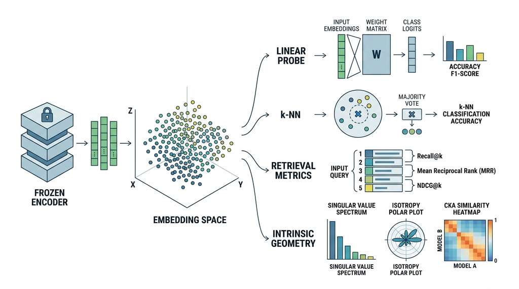
This philosophy aligns with how we evaluate discovery systems more broadly. In Chapter 6, we discussed how system architecture must be evaluated end-to-end against downstream objectives, not just component-level metrics. The same principle applies here: a representation is only as good as the tasks it enables. In short: an embedding you cannot probe, retrieve with, or geometrically inspect is an embedding you cannot trust.

2. Linear Probes

Choosing the wrong evaluation metric does not just give a misleading number; it can send an entire project down a dead end, burning months of compute on an encoder whose embeddings collapse the moment they meet a real downstream task. What follows is the standard toolkit for catching that failure before it costs you.

A linear probe is a single linear layer (plus optional bias) trained on top of frozen encoder features. The encoder is not updated during probe training; only the linear weights are optimized. If the probe achieves high accuracy, then the task-relevant information is linearly accessible in the representation space.

A linear probe fits a weight matrix \(W \in \mathbb{R}^{d \times C}\) and bias \(b \in \mathbb{R}^C\) that map each \(d\)-dimensional frozen embedding to \(C\) class logits, optimized with cross-entropy loss. The probe's simplicity acts as a controlled experiment: any accuracy gain over chance must come from the representation itself, not from the probe's modeling power. Use a linear probe when you want a cheap, reproducible score for comparing encoders or checkpoints. Switch to k-NN evaluation when the representation encodes useful structure in a nonlinear arrangement that no hyperplane can capture. Switch to retrieval metrics when your downstream application is search rather than classification.

The protocol is straightforward:

1. Encode all samples in the evaluation dataset using the frozen encoder.
2. Split into train and test sets.
3. Train a logistic regression (classification) or linear regression (regression) on the training embeddings.
4. Evaluate on the test embeddings.

import torch
import torch.nn as nn
import torch.nn.functional as F
from torch.utils.data import DataLoader, TensorDataset
from sklearn.linear_model import LogisticRegression
from sklearn.metrics import accuracy_score, f1_score
import numpy as np

class LinearProbe:
    """Evaluate representation quality via linear classification.

    Two implementations: scikit-learn (fast, for small datasets)
    and PyTorch (GPU-accelerated, for large datasets).
    """

    def __init__(self, method: str = 'sklearn'):
        self.method = method

    def evaluate_sklearn(self, train_features: np.ndarray,
                         train_labels: np.ndarray,
                         test_features: np.ndarray,
                         test_labels: np.ndarray) -> dict:
        """Fast linear probe using scikit-learn."""
        clf = LogisticRegression(
            max_iter=1000, C=1.0, solver='lbfgs',
            multi_class='multinomial'
        )
        clf.fit(train_features, train_labels)
        preds = clf.predict(test_features)

        return {
            'accuracy': accuracy_score(test_labels, preds),
            'f1_macro': f1_score(test_labels, preds, average='macro'),
            'f1_weighted': f1_score(test_labels, preds,
                                    average='weighted'),
        }

    def evaluate_pytorch(self, train_features: torch.Tensor,
                         train_labels: torch.Tensor,
                         test_features: torch.Tensor,
                         test_labels: torch.Tensor,
                         num_classes: int,
                         epochs: int = 100,
                         lr: float = 0.01) -> dict:
        """GPU-accelerated linear probe for large datasets."""
        dim = train_features.size(1)
        probe = nn.Linear(dim, num_classes)

        if torch.cuda.is_available():
            probe = probe.cuda()
            train_features = train_features.cuda()
            train_labels = train_labels.cuda()
            test_features = test_features.cuda()
            test_labels = test_labels.cuda()

        optimizer = torch.optim.Adam(probe.parameters(), lr=lr)
        dataset = TensorDataset(train_features, train_labels)
        loader = DataLoader(dataset, batch_size=256, shuffle=True)

        probe.train()
        for epoch in range(epochs):
            for batch_x, batch_y in loader:
                logits = probe(batch_x)
                loss = F.cross_entropy(logits, batch_y)
                optimizer.zero_grad()
                loss.backward()
                optimizer.step()

        probe.eval()
        with torch.no_grad():
            test_logits = probe(test_features)
            preds = test_logits.argmax(dim=1)
            acc = (preds == test_labels).float().mean().item()

        return {'accuracy': acc}

# Example: evaluate representations on a classification task
def run_linear_probe_demo():
    """Complete linear probe evaluation pipeline."""
    from sklearn.datasets import make_classification
    from sklearn.model_selection import train_test_split

    # Generate a synthetic dataset
    X, y = make_classification(
        n_samples=2000, n_features=128, n_informative=20,
        n_classes=5, random_state=42
    )

    # Simulate an encoder that produces 64-dim representations
    encoder_weights = np.random.randn(128, 64) * 0.1
    features = X @ encoder_weights  # simple linear projection

    # Split
    X_train, X_test, y_train, y_test = train_test_split(
        features, y, test_size=0.3, random_state=42
    )

    probe = LinearProbe(method='sklearn')
    results = probe.evaluate_sklearn(X_train, y_train, X_test, y_test)
    print("Linear Probe Results:")
    for metric, value in results.items():
        print(f"  {metric}: {value:.4f}")

    return results

results = run_linear_probe_demo()

3. k-NN Classification

Linear probes answer whether task information is accessible through a single hyperplane, but many useful representations organize their structure in ways that no flat boundary can capture; testing the local neighborhood around each point reveals what a global linear cut misses.

While linear probes test global linear separability, k-nearest-neighbor (k-NN) classifiers test the local geometry of the representation space. A k-NN classifier assigns a test sample the majority label among its \(k\) nearest neighbors in embedding space. It requires no training at all; the representation space is the entire model.

k-NN evaluation offers several advantages over linear probes: it is non-parametric (no hyperparameters beyond \(k\)), deterministic (no optimizer randomness), and extremely fast to run. It also captures local structure more faithfully. A representation where same-class samples form tight, well-separated clusters scores highly on k-NN even if the clusters are arranged non-linearly.

import torch
import numpy as np
from collections import Counter

def knn_evaluate(train_features: torch.Tensor,
                 train_labels: torch.Tensor,
                 test_features: torch.Tensor,
                 test_labels: torch.Tensor,
                 k_values: list = [1, 5, 10, 20],
                 metric: str = 'cosine') -> dict:
    """Evaluate representations using k-NN classification.

    Args:
        train_features: (N_train, D) reference embeddings
        train_labels: (N_train,) reference labels
        test_features: (N_test, D) query embeddings
        test_labels: (N_test,) query labels (ground truth)
        k_values: list of k values to evaluate
        metric: 'cosine' or 'euclidean'

    Returns:
        Dictionary mapping k -> accuracy
    """
    # Normalize for cosine similarity
    if metric == 'cosine':
        train_features = torch.nn.functional.normalize(
            train_features, dim=1
        )
        test_features = torch.nn.functional.normalize(
            test_features, dim=1
        )
        # For normalized vectors, cosine sim = dot product
        # Higher sim = more similar, so negate for "distance"
        sims = torch.mm(test_features, train_features.t())
        # Get top-k most similar (largest values)
        max_k = max(k_values)
        topk_sims, topk_indices = sims.topk(max_k, dim=1)
    else:
        # Euclidean: compute pairwise distances
        dists = torch.cdist(test_features, train_features)
        max_k = max(k_values)
        _, topk_indices = dists.topk(max_k, dim=1, largest=False)

    # Retrieve labels of nearest neighbors
    topk_labels = train_labels[topk_indices]  # (N_test, max_k)

    results = {}
    for k in k_values:
        # Majority vote among k nearest neighbors
        k_labels = topk_labels[:, :k]  # (N_test, k)
        preds = []
        for i in range(k_labels.size(0)):
            counter = Counter(k_labels[i].tolist())
            preds.append(counter.most_common(1)[0][0])
        preds = torch.tensor(preds)
        acc = (preds == test_labels).float().mean().item()
        results[f'knn_k{k}'] = acc

    return results

# Example: compare k-NN accuracy across representation qualities
dim = 64
n_train, n_test = 1000, 300
n_classes = 5

# Good representation: class-dependent structure
train_labels = torch.randint(0, n_classes, (n_train,))
test_labels = torch.randint(0, n_classes, (n_test,))

# Class centroids spread in space
centroids = torch.randn(n_classes, dim) * 3
train_feats = centroids[train_labels] + torch.randn(n_train, dim) * 0.5
test_feats = centroids[test_labels] + torch.randn(n_test, dim) * 0.5

results = knn_evaluate(train_feats, train_labels,
                       test_feats, test_labels)
print("k-NN Results (good representation):")
for metric, value in results.items():
    print(f"  {metric}: {value:.4f}")

# Poor representation: random features
train_random = torch.randn(n_train, dim)
test_random = torch.randn(n_test, dim)
results_bad = knn_evaluate(train_random, train_labels,
                           test_random, test_labels)
print("\nk-NN Results (random representation):")
for metric, value in results_bad.items():
    print(f"  {metric}: {value:.4f}")

4. Retrieval Metrics

For many scientific applications, the primary use of representations is retrieval: given a query (a molecule, an abstract, a spectrum), find the most similar items in a corpus. Retrieval quality is measured by metrics that capture whether the retrieved results are relevant and properly ranked.

The standard retrieval metrics are:

• Recall@k: What fraction of relevant items appear in the top \(k\) results? For example, Recall@10 measures whether the correct answer is within the first 10 retrieved items.
• Mean Reciprocal Rank (MRR): The average of \(1/\text{rank}\) across queries, where rank is the position of the first relevant result. MRR = 1.0 means the correct result is always first; MRR = 0.5 means it is typically second.
• Normalized Discounted Cumulative Gain (NDCG@k): A graded relevance metric that rewards having more relevant items higher in the ranking. Unlike Recall@k, NDCG accounts for the ordering of results within the top \(k\).

import torch
import torch.nn.functional as F
import numpy as np

def retrieval_metrics(query_embs: torch.Tensor,
                      corpus_embs: torch.Tensor,
                      query_labels: torch.Tensor,
                      corpus_labels: torch.Tensor,
                      k_values: list = [1, 5, 10, 50]) -> dict:
    """Compute retrieval metrics for learned representations.

    A retrieved item is "relevant" if it shares the query's label.

    Args:
        query_embs: (N_q, D) normalized query embeddings
        corpus_embs: (N_c, D) normalized corpus embeddings
        query_labels: (N_q,) query labels
        corpus_labels: (N_c,) corpus labels
        k_values: list of k for Recall@k

    Returns:
        Dictionary of retrieval metrics
    """
    # Similarity matrix
    sims = torch.mm(query_embs, corpus_embs.t())  # (N_q, N_c)

    # Rank all corpus items for each query (descending similarity)
    _, indices = sims.sort(dim=1, descending=True)

    # Relevance matrix: does retrieved item match query label?
    retrieved_labels = corpus_labels[indices]  # (N_q, N_c)
    relevance = (retrieved_labels == query_labels.unsqueeze(1))

    results = {}

    # Recall@k
    for k in k_values:
        recall = relevance[:, :k].any(dim=1).float().mean().item()
        results[f'recall@{k}'] = recall

    # Mean Reciprocal Rank
    # Find rank of first relevant item for each query
    first_relevant = torch.zeros(query_embs.size(0))
    for i in range(query_embs.size(0)):
        relevant_positions = relevance[i].nonzero(as_tuple=True)[0]
        if len(relevant_positions) > 0:
            first_relevant[i] = 1.0 / (relevant_positions[0].item() + 1)
    results['mrr'] = first_relevant.mean().item()

    # NDCG@10
    k_ndcg = min(10, corpus_embs.size(0))
    dcg = (relevance[:, :k_ndcg].float()
           / torch.log2(torch.arange(2, k_ndcg + 2).float())).sum(dim=1)

    # Ideal DCG: sort by relevance
    n_relevant = relevance.sum(dim=1).clamp(max=k_ndcg)
    ideal_dcg = (torch.ones(k_ndcg)
                 / torch.log2(torch.arange(2, k_ndcg + 2).float()))
    idcg = torch.zeros(query_embs.size(0))
    for i in range(query_embs.size(0)):
        n_rel = int(n_relevant[i].item())
        idcg[i] = ideal_dcg[:n_rel].sum()

    ndcg = (dcg / idcg.clamp(min=1e-10)).mean().item()
    results['ndcg@10'] = ndcg

    return results

# Example: retrieval evaluation
N_q, N_c, dim = 100, 5000, 64
n_classes = 20

# Generate structured embeddings
query_labels = torch.randint(0, n_classes, (N_q,))
corpus_labels = torch.randint(0, n_classes, (N_c,))
centroids = torch.randn(n_classes, dim) * 2

query_embs = F.normalize(
    centroids[query_labels] + torch.randn(N_q, dim) * 0.3, dim=1
)
corpus_embs = F.normalize(
    centroids[corpus_labels] + torch.randn(N_c, dim) * 0.3, dim=1
)

metrics = retrieval_metrics(query_embs, corpus_embs,
                            query_labels, corpus_labels)
print("Retrieval Metrics:")
for name, value in metrics.items():
    print(f"  {name}: {value:.4f}")

5. Intrinsic Geometry: Dimension, Isotropy, and Structure

Beyond task-specific evaluation, we can characterize the geometric structure of the representation space itself. These intrinsic metrics diagnose problems like dimensional collapse (using only a few dimensions), anisotropy (embeddings clustered in a narrow cone), and rank deficiency (the effective rank is much lower than the nominal dimension).

Effective Dimension

The effective dimension of a representation space measures how many dimensions the encoder actually uses. A 768-dimensional encoder that concentrates all information in 50 principal components has an effective dimension of approximately 50. Low effective dimension wastes capacity and may indicate training problems.

We measure effective dimension via the participation ratio (a measure of how evenly variance is spread across dimensions) of the singular value spectrum. Given representation matrix \(Z \in \mathbb{R}^{N \times d}\) with singular values \(\sigma_1 \geq \sigma_2 \geq \cdots \geq \sigma_d\), the participation ratio is:

When all singular values are equal, \(d_{\text{eff}} = d\) (full rank). When only one singular value is nonzero, \(d_{\text{eff}} = 1\) (complete collapse).

Isotropy

Isotropy measures whether embeddings are uniformly distributed in all directions or concentrated in a narrow cone. Anisotropic representations (those whose embeddings concentrate in a narrow cone rather than spreading uniformly, a pattern common in pretrained language models) use space inefficiently: most of the volume of the embedding space is empty, and cosine similarity is biased toward high values.

We quantify isotropy using the ratio of the minimum to maximum eigenvalue of the centered covariance matrix, or equivalently, the uniformity metric from Section 26.2.

import torch
import numpy as np

def representation_geometry(embeddings: torch.Tensor) -> dict:
    """Compute intrinsic geometric properties of a representation.

    Args:
        embeddings: (N, D) representation matrix (not normalized)

    Returns:
        Dictionary of geometric metrics
    """
    N, D = embeddings.shape

    # Center the embeddings
    centered = embeddings - embeddings.mean(dim=0, keepdim=True)

    # SVD for singular value analysis
    U, S, Vh = torch.linalg.svd(centered, full_matrices=False)

    # 1. Effective dimension (participation ratio)
    s_squared = S ** 2
    d_eff = (s_squared.sum() ** 2) / (s_squared ** 2).sum()

    # 2. Explained variance ratio
    variance_ratio = s_squared / s_squared.sum()
    cumvar_90 = (variance_ratio.cumsum(0) < 0.90).sum().item() + 1

    # 3. Isotropy: ratio of smallest to largest eigenvalue
    # (eigenvalues of covariance = squared singular values / N)
    eigenvalues = s_squared / (N - 1)
    isotropy_ratio = (eigenvalues[-1] / eigenvalues[0]).item()

    # 4. Average cosine similarity (anisotropy indicator)
    normed = torch.nn.functional.normalize(embeddings, dim=1)
    sim_matrix = torch.mm(normed, normed.t())
    mask = ~torch.eye(N, dtype=torch.bool, device=embeddings.device)
    avg_cosine = sim_matrix[mask].mean().item()

    # 5. Condition number of the representation matrix
    condition_number = (S[0] / S[min(N, D) - 1]).item()

    return {
        'effective_dim': d_eff.item(),
        'nominal_dim': D,
        'dim_utilization': d_eff.item() / D,
        'dims_for_90pct_var': cumvar_90,
        'isotropy_ratio': isotropy_ratio,
        'avg_cosine_sim': avg_cosine,
        'condition_number': condition_number,
    }

# Compare: isotropic vs anisotropic representations
print("Isotropic (random Gaussian):")
z_iso = torch.randn(1000, 128)
for k, v in representation_geometry(z_iso).items():
    print(f"  {k}: {v:.4f}" if isinstance(v, float)
          else f"  {k}: {v}")

print("\nAnisotropic (low effective rank):")
# Create a representation that uses only 10 of 128 dimensions
z_aniso = torch.randn(1000, 10) @ torch.randn(10, 128)
for k, v in representation_geometry(z_aniso).items():
    print(f"  {k}: {v:.4f}" if isinstance(v, float)
          else f"  {k}: {v}")

print("\nCollapsed (near-constant):")
z_collapsed = torch.ones(1000, 128) + 0.01 * torch.randn(1000, 128)
for k, v in representation_geometry(z_collapsed).items():
    print(f"  {k}: {v:.4f}" if isinstance(v, float)
          else f"  {k}: {v}")

Key Insight: The Anisotropy Problem in Language Models

Pretrained language models (BERT, GPT) produce highly anisotropic representations: token embeddings concentrate in a narrow cone of the embedding space, with average cosine similarity between random pairs reported in several studies to exceed 0.5, meaning any two randomly chosen sentences already look more alike than different. This means that cosine similarity between any two sentences is biased toward high values, making it difficult to distinguish genuinely similar sentences from dissimilar ones. Contrastive fine-tuning (as in Sentence-BERT and sentence-transformers) corrects this by spreading the representations uniformly over the hypersphere. This is exactly the uniformity objective from Section 26.2. When building domain-specific embedding models in Section 26.4, we will see how contrastive training transforms an anisotropic pretrained encoder into an isotropic one with dramatically improved retrieval performance.

6. Centered Kernel Alignment

The intrinsic geometry metrics above characterize a single representation space in isolation, but in practice you often need to ask a relational question: do two encoders, or two layers of the same encoder, organize the same data in the same way?

Comparing two representation spaces answers practical questions: have two encoders learned similar features? Has fine-tuning preserved the pretrained model's structure? Do different layers capture different aspects of the data?

Centered Kernel Alignment (CKA) provides a principled answer. Given two representation matrices \(X \in \mathbb{R}^{N \times p}\) and \(Y \in \mathbb{R}^{N \times q}\) (same \(N\) samples, possibly different dimensions), CKA measures the similarity of their kernel matrices:

where \(K_X = XX^\top\) and \(K_Y = YY^\top\) are the Gram matrices (matrices of all pairwise dot products between samples, capturing how similar each pair of inputs looks to a given encoder), and HSIC (Hilbert-Schmidt Independence Criterion) measures the dependence between the two kernel matrices after centering. CKA ranges from 0 (completely different structure) to 1 (identical structure up to rotation and scaling).

import torch

def centered_kernel_alignment(X: torch.Tensor,
                               Y: torch.Tensor) -> float:
    """Compute linear CKA between two representation matrices.

    Args:
        X: (N, p) first representation
        Y: (N, q) second representation

    Returns:
        CKA similarity score in [0, 1]
    """
    # Center both representations
    X = X - X.mean(dim=0, keepdim=True)
    Y = Y - Y.mean(dim=0, keepdim=True)

    # Linear kernels (Gram matrices)
    # HSIC with linear kernel simplifies to Frobenius inner products
    XtX = X.t() @ X  # (p, p)
    YtY = Y.t() @ Y  # (q, q)
    XtY = X.t() @ Y  # (p, q)

    # CKA = ||X^T Y||_F^2 / (||X^T X||_F * ||Y^T Y||_F)
    hsic_xy = (XtY ** 2).sum()
    hsic_xx = (XtX ** 2).sum()
    hsic_yy = (YtY ** 2).sum()

    cka = hsic_xy / (hsic_xx.sqrt() * hsic_yy.sqrt() + 1e-10)
    return cka.item()

def compare_layer_representations(model, data: torch.Tensor,
                                   layer_names: list) -> dict:
    """Compare CKA between all pairs of layer representations."""
    # Extract representations from each layer
    representations = {}
    hooks = []

    def make_hook(name):
        def hook(module, input, output):
            if isinstance(output, tuple):
                output = output[0]
            representations[name] = output.detach()
        return hook

    for name, module in model.named_modules():
        if name in layer_names:
            hooks.append(module.register_forward_hook(make_hook(name)))

    with torch.no_grad():
        model(data)

    for h in hooks:
        h.remove()

    # Compute pairwise CKA
    results = {}
    for i, name_i in enumerate(layer_names):
        for j, name_j in enumerate(layer_names):
            if j > i and name_i in representations \
                    and name_j in representations:
                xi = representations[name_i].flatten(1)
                xj = representations[name_j].flatten(1)
                cka = centered_kernel_alignment(xi, xj)
                results[f'{name_i} vs {name_j}'] = cka

    return results

# Example: CKA between random representations
X = torch.randn(500, 128)
Y_similar = X @ torch.randn(128, 64)  # linear transform of X
Y_different = torch.randn(500, 64)     # independent of X

cka_similar = centered_kernel_alignment(X, Y_similar)
cka_different = centered_kernel_alignment(X, Y_different)
print(f"CKA (linear transform): {cka_similar:.4f}")  # high
print(f"CKA (independent):      {cka_different:.4f}")  # low

7. Putting It Together: An Evaluation Dashboard

In practice, track multiple evaluation metrics simultaneously during representation learning. The following dashboard combines all the methods above.

import torch
import torch.nn.functional as F
import numpy as np
from dataclasses import dataclass, field

@dataclass
class EvalResults:
    """Container for comprehensive representation evaluation."""
    linear_probe_acc: float = 0.0
    knn_1_acc: float = 0.0
    knn_5_acc: float = 0.0
    recall_at_10: float = 0.0
    mrr: float = 0.0
    effective_dim: float = 0.0
    isotropy_ratio: float = 0.0
    avg_cosine: float = 0.0
    alignment: float = 0.0
    uniformity: float = 0.0

    def summary(self) -> str:
        lines = ["Representation Evaluation Dashboard",
                 "=" * 40]
        lines.append(f"Linear Probe Acc:   {self.linear_probe_acc:.4f}")
        lines.append(f"k-NN (k=1) Acc:     {self.knn_1_acc:.4f}")
        lines.append(f"k-NN (k=5) Acc:     {self.knn_5_acc:.4f}")
        lines.append(f"Recall@10:          {self.recall_at_10:.4f}")
        lines.append(f"MRR:                {self.mrr:.4f}")
        lines.append(f"Effective Dim:      {self.effective_dim:.1f}")
        lines.append(f"Isotropy Ratio:     {self.isotropy_ratio:.6f}")
        lines.append(f"Avg Cosine Sim:     {self.avg_cosine:.4f}")
        lines.append(f"Alignment:          {self.alignment:.4f}")
        lines.append(f"Uniformity:         {self.uniformity:.4f}")
        return "\n".join(lines)

def full_evaluation(encoder, train_data, train_labels,
                    test_data, test_labels,
                    positive_pairs=None) -> EvalResults:
    """Run the complete evaluation dashboard."""
    encoder.eval()
    with torch.no_grad():
        train_embs = encoder(train_data)
        test_embs = encoder(test_data)

    results = EvalResults()

    # Linear probe (sklearn for speed)
    from sklearn.linear_model import LogisticRegression
    clf = LogisticRegression(max_iter=500, C=1.0)
    clf.fit(train_embs.numpy(), train_labels.numpy())
    results.linear_probe_acc = clf.score(
        test_embs.numpy(), test_labels.numpy()
    )

    # k-NN
    normed_train = F.normalize(train_embs, dim=1)
    normed_test = F.normalize(test_embs, dim=1)
    sims = torch.mm(normed_test, normed_train.t())
    _, top_k = sims.topk(5, dim=1)

    # k=1
    preds_1 = train_labels[top_k[:, 0]]
    results.knn_1_acc = (preds_1 == test_labels).float().mean().item()

    # k=5
    from collections import Counter
    preds_5 = []
    for i in range(len(test_labels)):
        c = Counter(train_labels[top_k[i]].tolist())
        preds_5.append(c.most_common(1)[0][0])
    preds_5 = torch.tensor(preds_5)
    results.knn_5_acc = (preds_5 == test_labels).float().mean().item()

    # Intrinsic geometry
    centered = train_embs - train_embs.mean(0, keepdim=True)
    S = torch.linalg.svdvals(centered)
    s2 = S ** 2
    results.effective_dim = (s2.sum() ** 2 / (s2 ** 2).sum()).item()

    eig = s2 / (len(train_embs) - 1)
    results.isotropy_ratio = (eig[-1] / eig[0]).item()

    sim_all = torch.mm(normed_train, normed_train.t())
    mask = ~torch.eye(len(normed_train), dtype=torch.bool)
    results.avg_cosine = sim_all[mask].mean().item()

    # Alignment and uniformity (if positive pairs provided)
    if positive_pairs is not None:
        z1, z2 = positive_pairs
        z1 = F.normalize(z1, dim=1)
        z2 = F.normalize(z2, dim=1)
        results.alignment = (z1 - z2).norm(dim=1).pow(2).mean().item()
        sq_pdist = torch.pdist(z1, p=2).pow(2)
        results.uniformity = sq_pdist.mul(-2).exp().mean().log().item()

    encoder.train()
    return results

# Demo with a synthetic encoder
encoder = torch.nn.Sequential(
    torch.nn.Linear(64, 128), torch.nn.ReLU(),
    torch.nn.Linear(128, 32)
)

n_classes = 5
centroids = torch.randn(n_classes, 64) * 2
train_labels = torch.randint(0, n_classes, (500,))
test_labels = torch.randint(0, n_classes, (200,))
train_data = centroids[train_labels] + 0.5 * torch.randn(500, 64)
test_data = centroids[test_labels] + 0.5 * torch.randn(200, 64)

eval_results = full_evaluation(
    encoder, train_data, train_labels, test_data, test_labels
)
print(eval_results.summary())

When is pretraining "done enough"? Track the dashboard metrics across checkpoints. When linear probe accuracy, k-NN accuracy, and effective dimension all plateau for several consecutive checkpoints (typically 3 to 5 evaluations with no meaningful improvement), continued pretraining is unlikely to yield better representations. At that point, downstream fine-tuning (covered in Section 27.4) will typically deliver more value per compute hour than additional pretraining. If effective dimension is still rising while probe accuracy has stalled, the encoder is still reorganizing its internal structure and may benefit from a few more epochs; conversely, if effective dimension drops while probe accuracy holds, watch for early signs of dimensional collapse.

from sentence_transformers import SentenceTransformer
from sentence_transformers.evaluation import (
    InformationRetrievalEvaluator,
    EmbeddingSimilarityEvaluator,
)

model = SentenceTransformer("all-MiniLM-L6-v2")  # lightweight classic model

# Retrieval evaluation in 5 lines
evaluator = InformationRetrievalEvaluator(
    queries=queries, corpus=corpus, relevant_docs=qrels,
    name="sci-retrieval"
)
results = evaluator(model)
# Returns: recall@1, recall@5, recall@10, MRR, NDCG, MAP
# (MAP = Mean Average Precision, the mean of per-query
#  average precision across all relevant retrieved items)