38.2 GNNs for Knowledge Completion

1. From Static Embeddings to Message Passing

Aspirin inhibits COX-2, treats headaches, and irritates the stomach lining, yet TransE, RotatE, and ComplEx assign it one fixed vector that ignores all of that neighborhood context: entity \(e\) gets the same \(\mathbf{e}\) regardless of what query it appears in, as if the word "bank" received the same representation whether it appeared in "river bank" or "investment bank."

In 2020, researchers missed a promising COVID-19 drug repurposing candidate because their embedding model could not propagate evidence across the two-hop path from drug to shared protein target to disease. A neighborhood-aware model would have surfaced it automatically, because it encodes exactly that kind of multi-hop structural context into every entity's representation.

Graph neural networks resolve this by computing context-dependent entity representations through iterative message passing. At each layer \(l\), every node aggregates information from its neighbors and updates its own representation:

Each node collects and combines vector representations from its direct neighbors, then updates its own representation with the combined result. This procedure lets GNNs move beyond fixed per-entity embeddings: after each round, a node encodes its local graph structure, and after \(L\) rounds it has absorbed information from nodes up to \(L\) edges away. The mechanism applies a learnable transformation (typically a weight matrix followed by a nonlinearity) to each neighbor's vector, sums or averages the transformed vectors, and merges the result with the node's current state. Prefer message passing over static embeddings when entities have meaningful neighborhood structure (average degree above 5) and when multi-hop relational reasoning is required. Prefer embedding lookups (TransE, RotatE) when the graph is very sparse, the training budget is tight, or single-hop relational patterns suffice.

where \(\mathcal{N}(v)\) is the set of neighbors of node \(v\), AGGREGATE combines neighbor representations (typically by sum, mean, or attention-weighted combination), and UPDATE merges the aggregated neighborhood with the node's own representation (typically through a linear transform followed by a nonlinearity).

Multi-Hop Context

After \(L\) layers of message passing, each node's representation incorporates information from its \(L\)-hop neighborhood. With \(L=2\), the representation of Aspirin reflects not just its direct neighbors (COX-2, Headache) but also their neighbors (other COX-2 inhibitors, other headache treatments). This multi-hop context is precisely what makes GNNs powerful for link prediction: the model can learn that drugs sharing many target neighbors are likely to share yet-undiscovered targets. In short: a node does not need to see the whole graph; a few rounds of neighbor gossip let it reconstruct the structural role that static embeddings can only memorize.

2. R-GCN: Relational Graph Convolutional Networks

Standard GNNs treat all edges identically. In a knowledge graph, edges have types (inhibits, activates, binds_to), and each type carries different semantics. The Relational Graph Convolutional Network (R-GCN; Schlichtkrull et al., 2018) extends the GCN to multi-relational graphs by using relation-specific weight matrices.

The R-GCN update rule for node \(v\) at layer \(l\) is: Figure 38.2.1 illustrates R-GCN message passing with relation-specific weight matrices.

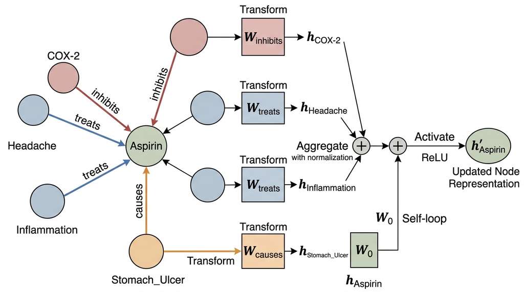
where \(\mathcal{N}_r(v)\) is the set of neighbors connected to \(v\) via relation \(r\), \(\mathbf{W}_r^{(l)}\) is the relation-specific weight matrix at layer \(l\), \(\mathbf{W}_0^{(l)}\) is the self-loop weight (preserving the node's own representation), and \(\sigma\) is a nonlinearity (typically ReLU). The normalization by \(|\mathcal{N}_r(v)|\) prevents nodes with many connections from dominating.

Figure 38.3 illustrates how one layer of R-GCN message passing aggregates neighbor information through relation-specific weight matrices before combining the results at the target node.

Over-smoothing constrains depth, but R-GCN faces a second, independent scaling challenge: the sheer number of parameters each layer introduces.

The core problem is parameter count. With \(|\mathcal{R}|\) relation types and \(d\)-dimensional hidden states, each layer contains \(|\mathcal{R}| \times d \times d\) parameters in the relation-specific weight matrices alone. A biomedical KG with 50 relation types and 256-dimensional hidden states produces \(50 \times 256 \times 256 \approx 3.3\) million parameters per layer. This volume invites overfitting on smaller graphs. R-GCN addresses it with two regularization strategies.

Basis decomposition represents each relation matrix as a linear combination of \(B\) shared basis matrices:

where \(\mathbf{V}_b^{(l)} \in \mathbb{R}^{d \times d}\) are shared basis matrices and \(a_{rb}^{(l)} \in \mathbb{R}\) are relation-specific coefficients. With \(B = 10\) basis matrices, the parameters per layer drop from \(|\mathcal{R}| \times d^2\) to \(B \times d^2 + |\mathcal{R}| \times B\), a reduction of roughly \(5\times\) for 50 relations.

Block-diagonal decomposition constrains each \(\mathbf{W}_r\) to be block-diagonal with \(B\) blocks of size \((d/B) \times (d/B)\). This reduces parameters by factor \(B\) and is computationally efficient but limits cross-dimension interactions within each relation transform.

import torch
import torch.nn as nn
import torch.nn.functional as F
from torch_geometric.nn import RGCNConv

class RGCNEncoder(nn.Module):
    """R-GCN encoder for knowledge graph entity representations."""

    def __init__(self, num_entities, num_relations, hidden_dim=128,
                 num_layers=2, num_bases=10, dropout=0.2):
        super().__init__()
        self.num_entities = num_entities
        self.num_relations = num_relations

        # Initial entity embeddings (learnable)
        self.entity_emb = nn.Embedding(num_entities, hidden_dim)
        nn.init.xavier_uniform_(self.entity_emb.weight)

        # Stack of R-GCN layers with basis decomposition
        self.convs = nn.ModuleList()
        for _ in range(num_layers):
            self.convs.append(
                RGCNConv(
                    in_channels=hidden_dim,
                    out_channels=hidden_dim,
                    num_relations=num_relations,
                    num_bases=num_bases,
                )
            )

        self.dropout = nn.Dropout(dropout)

    def forward(self, edge_index, edge_type):
        """
        Compute entity representations via message passing.

        Args:
            edge_index: [2, num_edges] source and target node indices
            edge_type: [num_edges] relation type for each edge

        Returns:
            Entity representations: [num_entities, hidden_dim]
        """
        x = self.entity_emb.weight  # (num_entities, hidden_dim)

        for i, conv in enumerate(self.convs):
            x = conv(x, edge_index, edge_type)
            if i < len(self.convs) - 1:  # no activation on last layer
                x = F.relu(x)
                x = self.dropout(x)

        return x


class RGCNLinkPredictor(nn.Module):
    """R-GCN encoder + DistMult decoder for link prediction."""

    def __init__(self, num_entities, num_relations, hidden_dim=128,
                 num_bases=10):
        super().__init__()
        self.encoder = RGCNEncoder(
            num_entities, num_relations, hidden_dim,
            num_bases=num_bases
        )
        # DistMult decoder: score = h^T diag(r) t
        self.relation_emb = nn.Embedding(num_relations, hidden_dim)
        nn.init.xavier_uniform_(self.relation_emb.weight)

    def encode(self, edge_index, edge_type):
        """Get entity representations from R-GCN."""
        return self.encoder(edge_index, edge_type)

    def decode(self, entity_embs, head_ids, rel_ids, tail_ids):
        """DistMult scoring: sum of element-wise h * r * t."""
        h = entity_embs[head_ids]
        r = self.relation_emb(rel_ids)
        t = entity_embs[tail_ids]
        return (h * r * t).sum(dim=-1)

    def forward(self, edge_index, edge_type,
                pos_triples, neg_triples):
        """Full forward pass: encode then decode."""
        entity_embs = self.encode(edge_index, edge_type)

        pos_scores = self.decode(
            entity_embs,
            pos_triples[:, 0], pos_triples[:, 1], pos_triples[:, 2]
        )
        neg_scores = self.decode(
            entity_embs,
            neg_triples[:, 0], neg_triples[:, 1], neg_triples[:, 2]
        )

        # Binary cross-entropy loss
        pos_loss = F.binary_cross_entropy_with_logits(
            pos_scores, torch.ones_like(pos_scores)
        )
        neg_loss = F.binary_cross_entropy_with_logits(
            neg_scores, torch.zeros_like(neg_scores)
        )
        return (pos_loss + neg_loss) / 2


# Example: small biomedical KG
num_entities = 8
num_relations = 4

# Graph structure: edges as (source, target) pairs with relation types
# Aspirin(0) -inhibits(0)-> COX-2(3)
# Ibuprofen(1) -inhibits(0)-> COX-1(2)
# Aspirin(0) -treats(1)-> Inflammation(4)
# Metformin(6) -activates(2)-> AMPK(7)
# Add reverse edges (R-GCN convention for undirected message passing)
edge_index = torch.tensor([
    [0, 3, 1, 2, 0, 4, 6, 7],  # sources
    [3, 0, 2, 1, 4, 0, 7, 6],  # targets
], dtype=torch.long)
edge_type = torch.tensor(
    [0, 0, 0, 0, 1, 1, 2, 2], dtype=torch.long
)

model = RGCNLinkPredictor(num_entities, num_relations, hidden_dim=64)

pos = torch.tensor([[0, 0, 3], [6, 2, 7]])
neg = torch.tensor([[0, 0, 7], [6, 2, 2]])

loss = model(edge_index, edge_type, pos, neg)
print(f"R-GCN + DistMult loss: {loss.item():.4f}")

3. The Encoder-Decoder Architecture

The R-GCN link predictor in Listing 38.5 follows the general encoder-decoder pattern: the encoder (R-GCN) aggregates neighborhood information into context-aware entity representations, and the decoder (DistMult here) scores candidate triples against those representations. Separating the two stages lets practitioners mix and match encoders and decoders independently.

Encoder choices determine how neighborhood information is aggregated:

• R-GCN: relation-specific linear transforms with basis decomposition. Simple and effective for small to medium graphs (up to ~100K nodes).
• CompGCN (Vashishth et al., 2020): jointly embeds entities and relations by composing them together before aggregation (for example, adding or multiplying a relation vector with a neighbor vector, so the message itself encodes the relation type rather than relying on a separate weight matrix). Supports TransE, RotatE, and DistMult composition operators within the GNN framework.
• GAT with relation types: attention-weighted aggregation where the attention mechanism is conditioned on the relation type. Learns which neighbors are most informative for each relation context.
• GraphSAGE with sampling: samples a fixed-size neighborhood at each layer, enabling training on graphs with millions of nodes by controlling memory consumption.

Decoder choices determine how the encoded representations are combined to score triples:

• DistMult: \(f(h, r, t) = \mathbf{h}^T \text{diag}(\mathbf{r}) \mathbf{t} = \sum_i h_i r_i t_i\). Simple and symmetric; best when combined with a GNN encoder that already captures directionality.
• TransE decoder: \(f(h, r, t) = -\|\mathbf{h} + \mathbf{r} - \mathbf{t}\|\). Uses the GNN-computed \(\mathbf{h}\) and \(\mathbf{t}\) with a separate relation embedding \(\mathbf{r}\).
• ConvE (Dettmers et al., 2018): reshapes head and relation embeddings into 2D "images" (by arranging the 1D embedding vector into a matrix, creating a spatial layout that 2D convolutions can slide over) and applies convolutional filters, then computes a dot product with the tail. Captures non-linear interactions at the cost of interpretability.

4. Training GNNs on Knowledge Graphs

Training a GNN for link prediction requires several considerations beyond standard supervised learning. The graph structure serves dual roles: it defines the message passing computation graph (encoder input) and provides the training supervision (positive triples). This creates a data leakage risk: if we include a test triple in the message passing graph, the model can predict it by looking up the direct edge.

The standard solution is edge masking (not to be confused with the inductive setting discussed later, where entirely new entities appear at test time). During training, we randomly drop a fraction of edges from the message passing graph and use those dropped edges as positive training triples. This forces the model to predict edges from indirect evidence (multi-hop paths) rather than direct observation. At evaluation time, we use the full graph for message passing but evaluate on held-out test triples.

import torch
from torch.optim import Adam
from torch_geometric.nn import RGCNConv
import numpy as np

def train_rgcn_link_prediction(
    model, edge_index, edge_type, all_triples,
    num_entities, num_epochs=100, lr=0.01,
    neg_ratio=10, val_fraction=0.1
):
    """
    Training loop for R-GCN link prediction.

    Args:
        model: RGCNLinkPredictor instance
        edge_index: full graph edge_index [2, num_edges]
        edge_type: relation types [num_edges]
        all_triples: tensor of all (h, r, t) triples
        num_entities: total entity count
        num_epochs: training epochs
        lr: learning rate
        neg_ratio: negatives per positive triple
        val_fraction: fraction of triples for validation
    """
    optimizer = Adam(model.parameters(), lr=lr, weight_decay=1e-5)

    # Split triples into train/val
    n = len(all_triples)
    perm = torch.randperm(n)
    val_size = int(n * val_fraction)
    val_triples = all_triples[perm[:val_size]]
    train_triples = all_triples[perm[val_size:]]

    # Known triple set for filtered evaluation
    known_set = set(
        (h.item(), r.item(), t.item())
        for h, r, t in all_triples
    )

    best_mrr = 0.0

    for epoch in range(num_epochs):
        model.train()

        # Generate negative samples by corrupting tails
        neg_tails = torch.randint(
            0, num_entities,
            (len(train_triples) * neg_ratio,)
        )
        neg_triples = train_triples.repeat(neg_ratio, 1)
        neg_triples[:, 2] = neg_tails

        # Edge dropout: remove 10% of edges during training
        keep_mask = torch.rand(edge_index.size(1)) > 0.1
        train_edge_index = edge_index[:, keep_mask]
        train_edge_type = edge_type[keep_mask]

        # Forward pass
        loss = model(
            train_edge_index, train_edge_type,
            train_triples, neg_triples
        )

        # Backward pass
        optimizer.zero_grad()
        loss.backward()
        torch.nn.utils.clip_grad_norm_(model.parameters(), 1.0)
        optimizer.step()

        # Validation every 10 epochs
        if (epoch + 1) % 10 == 0:
            model.eval()
            with torch.no_grad():
                entity_embs = model.encode(edge_index, edge_type)

                ranks = []
                for triple in val_triples[:100]:  # sample for speed
                    h, r, t = triple
                    # Score all tails
                    all_tails = torch.arange(num_entities)
                    scores = model.decode(
                        entity_embs,
                        h.expand(num_entities),
                        r.expand(num_entities),
                        all_tails,
                    )
                    # Filtered: mask known triples
                    for e in range(num_entities):
                        if e != t.item() and (h.item(), r.item(), e) in known_set:
                            scores[e] = float('-inf')

                    rank = (scores >= scores[t.item()]).sum().item()
                    ranks.append(rank)

                mrr = np.mean([1.0 / r for r in ranks])
                hits10 = np.mean([1.0 if r <= 10 else 0.0 for r in ranks])

                print(f"Epoch {epoch+1:3d} | Loss: {loss.item():.4f} "
                      f"| Val MRR: {mrr:.4f} | Hits@10: {hits10:.4f}")

                if mrr > best_mrr:
                    best_mrr = mrr
                    torch.save(model.state_dict(), "best_rgcn.pt")

    print(f"\nBest validation MRR: {best_mrr:.4f}")
    return model

5. Scalability: Mini-Batching and Neighbor Sampling

The R-GCN implementations above compute representations for all entities simultaneously. This is feasible for graphs with tens of thousands of nodes, but scientific knowledge graphs can contain millions of entities. Hetionet has 47,000 nodes; Wikidata has over 100 million. Full-graph message passing on such graphs exhausts GPU memory.

The solution is neighbor sampling (Hamilton et al., 2017), which constructs a mini-batch computation graph by sampling a fixed number of neighbors per node at each layer. For a 2-layer GNN with 15 sampled neighbors per layer, the computation graph for a batch of 1024 target nodes includes at most \(1024 \times 15 = 15{,}360\) first-hop neighbors and \(15{,}360 \times 15 = 230{,}400\) second-hop neighbors, a 225x expansion from the original batch size in just two hops. This bounded computation graph fits in GPU memory regardless of the full graph size.

from torch_geometric.loader import NeighborLoader
from torch_geometric.data import Data

def create_kg_dataloader(edge_index, edge_type, num_nodes,
                          batch_size=1024, num_neighbors=[15, 10]):
    """
    Create a neighbor-sampling dataloader for scalable GNN training.

    Args:
        edge_index: [2, num_edges] graph connectivity
        edge_type: [num_edges] relation types
        num_nodes: total nodes in graph
        batch_size: number of target nodes per batch
        num_neighbors: neighbors to sample at each GNN layer
    """
    # Wrap graph in PyG Data object
    data = Data(
        edge_index=edge_index,
        edge_type=edge_type,
        num_nodes=num_nodes,
    )

    # NeighborLoader samples subgraphs around target nodes
    loader = NeighborLoader(
        data,
        num_neighbors=num_neighbors,  # [15 first-hop, 10 second-hop]
        batch_size=batch_size,
        shuffle=True,
        num_workers=4,
    )

    return loader


# Example: iterate over mini-batches of a large KG
# (using our small example; scales to millions of nodes)
loader = create_kg_dataloader(
    edge_index, edge_type,
    num_nodes=num_entities,
    batch_size=4,
    num_neighbors=[3, 2]
)

for batch in loader:
    print(f"Batch: {batch.num_nodes} nodes, "
          f"{batch.edge_index.size(1)} edges")
    # batch.n_id maps local node IDs to global IDs
    # batch.edge_index uses local IDs within the subgraph
    # batch.batch_size gives the number of target nodes
    break

The trade-off is variance: each mini-batch sees a random sample of each node's neighborhood, so gradient estimates are noisier than full-graph computation. In practice, neighbor sampling with 10 to 25 neighbors per layer captures sufficient structural information for most knowledge graph tasks, typically with only modest accuracy loss compared to full-graph training.

6. GNN vs. Embedding-Only: When to Use Each

Neighbor sampling and mini-batching solve the memory problem, but they raise a practical question: given the extra engineering and compute cost, when is a GNN encoder actually worth it? GNN encoders are not always superior to static embeddings. The choice depends on graph structure, available features, and computational budget.

Use GNN encoders when:

• Entities have rich features: gene expression profiles, molecular fingerprints, or textual descriptions. GNNs can incorporate these features as initial node representations, while embedding-only models must learn everything from graph structure alone.
• Multi-hop reasoning is needed: the target relation requires integrating information across 2+ hops. Drug repurposing (drug to target to pathway to disease) is the canonical example.
• The graph is dense and well-connected: message passing provides diminishing returns when nodes have few neighbors. A GNN on a sparse graph (average degree < 5) often underperforms RotatE.
• Inductive prediction is required: GNNs can generate representations for new entities not seen during training (if those entities have features and some known edges), while embedding-only models require retraining.

Use embedding-only models (TransE, RotatE, ComplEx) when:

• The graph is large but sparse: millions of entities with low average degree. Embedding lookups are \(O(1)\) regardless of graph size.
• Training budget is limited: embedding models typically train 5 to 10 times faster than GNN models on the same graph because they avoid message passing computation.
• Relations have clear geometric patterns: if most relations are antisymmetric with compositional structure, RotatE captures these patterns directly without the overhead of GNN layers.
• Entities lack informative features: when the only information is the graph structure itself, GNN encoders reduce to embedding lookups with extra computation. The basis decomposition in R-GCN partially mitigates this, but the benefit over RotatE is modest.

7. Attention-Based Message Passing for Knowledge Graphs

The hybrid insight points to a deeper question: if some neighbors matter more than others for a given prediction, can the model learn to weight them accordingly? Not all neighbors are equally informative. When predicting a drug's therapeutic effect, its binding targets are more relevant than its metabolic enzymes. Graph Attention Networks (GAT; Velickovic et al., 2018) learn attention weights that control how much each neighbor contributes to the aggregated message.

For knowledge graphs, we extend attention to be relation-aware. The attention coefficient between node \(v\) and neighbor \(u\) connected by relation \(r\) is:

where \(\mathbf{a}\) is a learnable attention vector and \(\|\) denotes concatenation. The aggregation then uses these attention weights:

The attention weights are interpretable: after training, we can inspect which neighbors and relation types the model considers most important for each prediction. This interpretability is valuable in scientific applications where researchers want to understand not just the prediction but the reasoning path behind it.

import torch
import torch.nn as nn
import torch.nn.functional as F

class RelationalGATLayer(nn.Module):
    """A single layer of relation-aware graph attention."""

    def __init__(self, in_dim, out_dim, num_relations, num_heads=4):
        super().__init__()
        self.num_heads = num_heads
        self.head_dim = out_dim // num_heads

        # Relation-specific projections
        self.W = nn.ModuleList([
            nn.Linear(in_dim, out_dim, bias=False)
            for _ in range(num_relations)
        ])

        # Attention parameters (shared across relations)
        self.attn = nn.Parameter(
            torch.randn(num_heads, 2 * self.head_dim)
        )
        nn.init.xavier_uniform_(self.attn.unsqueeze(0))

    def forward(self, x, edge_index, edge_type):
        """
        Args:
            x: node features [num_nodes, in_dim]
            edge_index: [2, num_edges]
            edge_type: [num_edges]
        Returns:
            Updated node features [num_nodes, out_dim]
        """
        src, dst = edge_index
        num_nodes = x.size(0)

        # Apply relation-specific transforms to source nodes
        h_src = torch.zeros(edge_index.size(1), self.num_heads,
                            self.head_dim, device=x.device)
        h_dst = torch.zeros_like(h_src)

        for r in range(len(self.W)):
            mask = edge_type == r
            if mask.any():
                projected = self.W[r](x).view(-1, self.num_heads,
                                               self.head_dim)
                h_src[mask] = projected[src[mask]]
                h_dst[mask] = projected[dst[mask]]

        # Compute attention: concat source and target, dot with attn
        attn_input = torch.cat([h_src, h_dst], dim=-1)  # [E, H, 2*d]
        attn_scores = (attn_input * self.attn).sum(dim=-1)  # [E, H]
        attn_scores = F.leaky_relu(attn_scores, 0.2)

        # Softmax over incoming edges for each target node
        attn_weights = torch.zeros(num_nodes, edge_index.size(1),
                                    self.num_heads, device=x.device)
        # Scatter softmax (simplified; use torch_scatter in production)
        attn_scores = attn_scores - attn_scores.max()
        exp_scores = torch.exp(attn_scores)  # [E, H]

        # Weighted aggregation
        weighted = h_src * exp_scores.unsqueeze(-1)  # [E, H, d]

        # Sum messages to target nodes
        out = torch.zeros(num_nodes, self.num_heads, self.head_dim,
                          device=x.device)
        out.scatter_add_(0, dst.unsqueeze(-1).unsqueeze(-1).expand_as(weighted),
                         weighted)

        # Normalize by sum of attention weights
        norm = torch.zeros(num_nodes, self.num_heads, 1,
                           device=x.device)
        norm.scatter_add_(0, dst.unsqueeze(-1).unsqueeze(-1).expand(
            -1, self.num_heads, 1), exp_scores.unsqueeze(-1))
        out = out / (norm + 1e-12)

        return out.view(num_nodes, -1)  # [num_nodes, out_dim]


# Example: 4-head relational attention
gat_layer = RelationalGATLayer(
    in_dim=64, out_dim=64, num_relations=4, num_heads=4
)
x = torch.randn(8, 64)  # 8 entities, 64-dim features
out = gat_layer(x, edge_index, edge_type)
print(f"Input: {x.shape} -> Output: {out.shape}")

from torch_geometric.nn import RGCNConv, GATConv, Sequential
from torch_geometric.data import Data

# 2-layer R-GCN in 6 lines
model = Sequential('x, edge_index, edge_type', [
    (RGCNConv(128, 128, num_relations=50, num_bases=10),
     'x, edge_index, edge_type -> x'),
    (nn.ReLU(), 'x -> x'),
    (RGCNConv(128, 128, num_relations=50, num_bases=10),
     'x, edge_index, edge_type -> x'),
])

# PyG handles sparse message passing, GPU batching,
# neighbor sampling, and distributed training internally.
# This replaces ~150 lines of custom aggregation code.

Exercises

1. (Conceptual) Explain why a 2-layer R-GCN can capture the reasoning pattern "Drug X inhibits Protein Y, and Protein Y is involved in Disease Z, therefore Drug X may treat Disease Z," while a single-layer R-GCN cannot. What does a 3-layer R-GCN capture that 2 layers miss?
2. (Coding) Implement a CompGCN layer that composes relation embeddings into the message passing using the RotatE composition operator (element-wise complex multiplication). Compare link prediction MRR against the R-GCN + DistMult model from Listing 38.5 on the FB15k-237 dataset (available in PyKEEN or PyG).
3. (Analysis) Train the R-GCN link predictor from Listing 38.6 with 1, 2, 3, and 4 layers on a biomedical KG subset (use the Drug Repurposing Knowledge Graph (DRKG) dataset from AWS). Plot MRR versus number of layers. At what depth does over-smoothing begin to degrade performance? Add skip connections (residual connections) and measure whether they mitigate the degradation.