Prerequisites
This section builds on the embedding space concepts from Chapter 26: Representation Learning, particularly the idea that geometric relationships in learned vector spaces can encode semantic meaning. You should be comfortable with complex numbers (magnitude, phase, conjugate), dot products, and the L1/L2 norms. The knowledge representation foundations from Chapter 3 provide the conceptual grounding for why we represent knowledge as triples.
A knowledge graph is a collection of (head, relation, tail) triples: (Aspirin, inhibits, COX-2), (TP53, activates, Apoptosis), (Graphene, exhibits, High_Conductivity). Link prediction asks: given a partially observed graph, which unobserved triples are likely true? This is the core question for scientific discovery, because every missing edge is a potential hypothesis. The approach is to embed entities and relations into a continuous vector space where a simple geometric test (a translation, a rotation, a dot product) scores how plausible any given triple is. We train these embeddings on known triples and then rank all possible missing triples by their scores. The top-ranked missing links become discovery candidates.
1. The Link Prediction Problem
In 2020, a graph embedding model scored every drug in a biomedical database against the query "treats SARS-CoV-2 infection." It ranked baricitinib, a rheumatoid arthritis medication, among the top candidates. Within months, baricitinib received emergency authorization for COVID-19 treatment. The technique behind that prediction, link prediction, starts from a deceptively simple formulation. Let \(\mathcal{E}\) be a set of entities and \(\mathcal{R}\) a set of relation types. A knowledge graph \(\mathcal{G} \subset \mathcal{E} \times \mathcal{R} \times \mathcal{E}\) is a set of observed triples \((h, r, t)\) where \(h\) is the head entity, \(r\) is the relation, and \(t\) is the tail entity. The link prediction task is: given a query $(h, r, ?)$ or $(?, r, t)$, rank all candidate entities by the likelihood that the completed triple is true.
Link prediction is a ranking problem over the full entity vocabulary. Given an incomplete triple with one slot missing, a model assigns a plausibility score to every candidate entity and sorts them from most to least likely. It matters because scientific knowledge graphs are always dramatically incomplete: curated databases capture a small fraction of real biological or chemical interactions. Ranking the missing edges systematically surfaces testable hypotheses at scale. The model learns a low-dimensional vector for each entity and each relation type, then applies a geometric scoring function (vector addition, rotation, or dot product) that returns high values for combinations consistent with observed patterns and low values otherwise. Link prediction fits when you have a structured graph of typed relationships and want to prioritize which unobserved relationships to investigate experimentally. For unstructured text or single-relation networks, retrieval models or graph algorithms (such as label propagation) work better.
In scientific knowledge graphs, the entities are biological molecules, genes, diseases, chemical compounds, materials, or physical phenomena. The relations encode scientific interactions: causes, inhibits, activates, binds_to, treats, upregulates, is_substrate_of. A biomedical knowledge graph might contain triples like:
- (Metformin, treats, Type_2_Diabetes)
- (BRCA1, associated_with, Breast_Cancer)
- (Ibuprofen, inhibits, COX-1)
- (TNF-alpha, activates, NF-kB)
- (Penicillin, binds_to, PBP2)
The key insight is that these graphs are always incomplete. DrugBank contains roughly 15,000 drug-target interactions (circa 2020), but the true number of pharmacologically relevant interactions is estimated to be orders of magnitude larger. Every curated database represents a lower bound on the true set of relations. Link prediction aims to fill in the gaps. In short: every absent edge in a knowledge graph is not a denial but an uninvestigated hypothesis, and embedding models let you rank millions of those hypotheses by geometric plausibility in seconds.
The Open World Assumption distinguishes knowledge graphs from relational databases. In a database, if a row is absent, the fact is false (Closed World Assumption). In a knowledge graph, an absent triple simply means we do not know yet. This distinction is what makes link prediction meaningful for discovery: an absent edge between Drug X and Disease Y is not evidence against the relationship; it is an unstudied hypothesis. The embedding model's job is to estimate which unstudied hypotheses are most likely to be true, based on patterns in the observed graph.
Common Misconception
A frequent misconception is that a high link prediction score means the predicted relationship is probably true in reality. It does not. A high score means the predicted triple is structurally consistent with the patterns in the observed graph; it tells you nothing about whether the underlying biology or chemistry actually holds. Link prediction identifies statistically plausible hypotheses, not confirmed facts, and every top-ranked prediction still requires experimental validation before it can be treated as established knowledge.
2. TransE: Relations as Translations
When a drug repurposing pipeline uses the wrong embedding geometry, it silently misranks every symmetric interaction in the graph, burying valid protein-protein binding candidates below nonsense predictions. The choice of scoring function determines which entire categories of scientific relationships your model can represent at all.
The simplest and most influential knowledge graph embedding model is TransE (Bordes et al., 2013). The idea is elegant: if (h, r, t) is a true triple, then the embedding of the head entity plus the embedding of the relation should be close to the embedding of the tail entity. In vector notation:
$$\mathbf{h} + \mathbf{r} \approx \mathbf{t}$$The scoring function measures how well this translation property holds. Figure 38.1.1 illustrates TransE vs RotatE geometric scoring comparison.
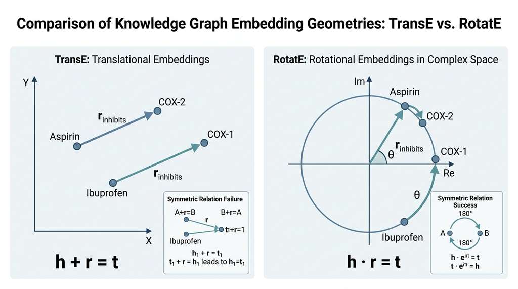
where \(\|\cdot\|_p\) is the L1 or L2 norm. Higher scores (closer to zero) indicate more plausible triples. For a true triple like (Aspirin, inhibits, COX-2), training pushes \(\mathbf{h}_{\text{aspirin}} + \mathbf{r}_{\text{inhibits}}\) toward \(\mathbf{t}_{\text{COX-2}}\). After training, we can query \((?, \text{inhibits}, \text{COX-2})\) by computing \(\mathbf{t}_{\text{COX-2}} - \mathbf{r}_{\text{inhibits}}\) and finding the nearest entity embeddings, discovering other potential COX-2 inhibitors.
TransE has a fundamental limitation: it cannot model symmetric relations. If (Drug_A, interacts_with, Drug_B) is true, TransE requires \(\mathbf{h}_A + \mathbf{r} \approx \mathbf{t}_B\) and \(\mathbf{h}_B + \mathbf{r} \approx \mathbf{t}_A\). This forces \(\mathbf{h}_A \approx \mathbf{t}_A\) and \(\mathbf{h}_B \approx \mathbf{t}_B\), collapsing the embeddings of interacting entities. It also struggles with one-to-many relations (one gene activating multiple pathways), because the translation from one head must land near multiple distinct tails.
Figure 38.1 below illustrates the geometric intuition behind all three scoring functions covered in this section: TransE's vector addition, RotatE's complex-plane rotation, and ComplEx's asymmetric dot product. Understanding these three geometries is the key to choosing the right model for a given knowledge graph.
import torch
import torch.nn as nn
import torch.nn.functional as F

class TransE(nn.Module):
    """TransE: knowledge graph embeddings via translation."""

    def __init__(self, num_entities, num_relations, embedding_dim=128):
        super().__init__()
        self.entity_embeddings = nn.Embedding(num_entities, embedding_dim)
        self.relation_embeddings = nn.Embedding(num_relations, embedding_dim)

        # Initialize with uniform distribution (Bordes et al., 2013)
        nn.init.uniform_(self.entity_embeddings.weight, -6.0/embedding_dim**0.5,
                         6.0/embedding_dim**0.5)
        nn.init.uniform_(self.relation_embeddings.weight, -6.0/embedding_dim**0.5,
                         6.0/embedding_dim**0.5)
        # Normalize relation embeddings to unit length
        with torch.no_grad():
            self.relation_embeddings.weight.data = F.normalize(
                self.relation_embeddings.weight.data, p=2, dim=1
            )

    def score(self, head_ids, relation_ids, tail_ids):
        """Score triples: higher (less negative) = more plausible."""
        h = self.entity_embeddings(head_ids)
        r = self.relation_embeddings(relation_ids)
        t = self.entity_embeddings(tail_ids)
        # Negative L1 distance: h + r should be close to t
        return -torch.norm(h + r - t, p=1, dim=-1)

    def forward(self, pos_triples, neg_triples, margin=1.0):
        """Margin-based ranking loss: push positive above negative."""
        pos_scores = self.score(
            pos_triples[:, 0], pos_triples[:, 1], pos_triples[:, 2]
        )
        neg_scores = self.score(
            neg_triples[:, 0], neg_triples[:, 1], neg_triples[:, 2]
        )
        # Margin loss: want pos_score > neg_score + margin
        loss = F.relu(margin - pos_scores + neg_scores).mean()
        return loss


# Example: a small biomedical knowledge graph
entities = ["Aspirin", "Ibuprofen", "COX-1", "COX-2",
            "Inflammation", "Pain", "Metformin", "AMPK"]
relations = ["inhibits", "treats", "activates", "binds_to"]

model = TransE(
    num_entities=len(entities),
    num_relations=len(relations),
    embedding_dim=64
)

# Positive triples: (head_id, relation_id, tail_id)
pos = torch.tensor([
    [0, 0, 3],  # Aspirin inhibits COX-2
    [1, 0, 2],  # Ibuprofen inhibits COX-1
    [0, 1, 4],  # Aspirin treats Inflammation
    [6, 2, 7],  # Metformin activates AMPK
])

# Negative triples: corrupt tail entity
neg = torch.tensor([
    [0, 0, 7],  # Aspirin inhibits AMPK (false)
    [1, 0, 5],  # Ibuprofen inhibits Pain (false)
    [0, 1, 7],  # Aspirin treats AMPK (false)
    [6, 2, 2],  # Metformin activates COX-1 (false)
])

loss = model(pos, neg, margin=1.0)
print(f"TransE margin loss: {loss.item():.4f}")
3. RotatE: Relations as Rotations in Complex Space
RotatE (Sun et al., 2019) addresses TransE's limitations by modeling relations as element-wise rotations in complex vector space. Each entity is embedded as a complex vector \(\mathbf{h}, \mathbf{t} \in \mathbb{C}^d\), and each relation is a complex vector \(\mathbf{r} \in \mathbb{C}^d\) with unit modulus (each component has magnitude exactly 1, meaning it lies on the unit circle in the complex plane): \(|r_i| = 1\) for each component. The scoring function is:
$$f_{\text{RotatE}}(h, r, t) = -\|\mathbf{h} \circ \mathbf{r} - \mathbf{t}\|$$where \(\circ\) denotes the Hadamard (element-wise) product, where each component of the first vector is multiplied by the corresponding component of the second. Since each \(r_i = e^{i\theta_i}\) is a point on the unit circle, multiplying by \(r_i\) rotates \(h_i\) by angle \(\theta_i\) in the complex plane. This seemingly small change has profound consequences for expressiveness:
- Symmetric relations (interacts_with): set \(\theta_i = 0\) or \(\pi\), so \(r_i = \pm 1\) and rotation is its own inverse.
- Antisymmetric relations (inhibits): use arbitrary \(\theta_i \neq 0, \pi\), so the forward and reverse rotations differ.
- Inversion: if \(r_1\) is the rotation for "inhibits" and \(r_2\) for "is_inhibited_by", then \(r_2 = \bar{r}_1\) (complex conjugate, i.e., reverse rotation).
- Composition: if "A causes B" and "B causes C" imply "A causes C", the rotation for the composed relation is the product of individual rotations: \(r_{\text{causes}} \circ r_{\text{causes}} = r_{\text{causes}}^2\).
Mental Model
Think of RotatE like a combination lock with 128 independent dials. Each entity is described by the position of all 128 dials, and each relation type is a specific set of turns (one per dial). To check whether "Aspirin inhibits COX-2," you start at Aspirin's dial positions, apply the "inhibits" turns, and see whether you land close to COX-2's dial positions. Symmetric relations (like "interacts_with") correspond to turns that are either zero or a full half-turn, so applying them twice returns you to where you started. Antisymmetric relations use intermediate turn amounts, so applying and then reversing them does not cancel out. The key mechanism that makes this more powerful than TransE's simple shift: each of the 128 dials turns independently, giving the model a combinatorial space of possible relation signatures rather than a single direction.
TransE encodes each relation as a single direction in vector space. This means two different relations that share the same head and tail must point the same direction, creating conflicts when the graph has multiple relation types between the same entity pairs. RotatE encodes each relation as a rotation angle per dimension, giving it \(d\) independent degrees of freedom. A 128-dimensional RotatE model can represent \(2^{128}\) distinct relation patterns, because each dimension independently rotates by a different angle. This combinatorial expressiveness is why RotatE consistently outperforms TransE on benchmarks with complex relational patterns.
import torch
import torch.nn as nn
import numpy as np

class RotatE(nn.Module):
    """RotatE: relations as rotations in complex embedding space."""

    def __init__(self, num_entities, num_relations, embedding_dim=128):
        super().__init__()
        # Entity embeddings: complex, stored as 2*dim reals
        self.entity_re = nn.Embedding(num_entities, embedding_dim)
        self.entity_im = nn.Embedding(num_entities, embedding_dim)

        # Relation embeddings: phase angles (constrained to unit modulus)
        self.relation_phase = nn.Embedding(num_relations, embedding_dim)

        self.embedding_dim = embedding_dim
        self.gamma = nn.Parameter(torch.tensor(12.0))  # margin

        # Xavier initialization
        nn.init.xavier_uniform_(self.entity_re.weight)
        nn.init.xavier_uniform_(self.entity_im.weight)
        nn.init.uniform_(self.relation_phase.weight,
                         -np.pi, np.pi)

    def score(self, head_ids, relation_ids, tail_ids):
        """Score = gamma - ||h * r - t|| in complex space."""
        # Head entity as complex vector
        h_re = self.entity_re(head_ids)
        h_im = self.entity_im(head_ids)

        # Relation as unit-modulus complex: r = cos(phase) + i*sin(phase)
        phase = self.relation_phase(relation_ids)
        r_re = torch.cos(phase)
        r_im = torch.sin(phase)

        # Tail entity as complex vector
        t_re = self.entity_re(tail_ids)
        t_im = self.entity_im(tail_ids)

        # Complex multiplication: (h_re + i*h_im)(r_re + i*r_im)
        hr_re = h_re * r_re - h_im * r_im
        hr_im = h_re * r_im + h_im * r_re

        # Distance in complex space
        diff_re = hr_re - t_re
        diff_im = hr_im - t_im
        distance = torch.sqrt(diff_re**2 + diff_im**2 + 1e-12).sum(dim=-1)

        return self.gamma - distance

    def forward(self, pos_triples, neg_triples):
        """Self-adversarial negative sampling loss (Sun et al., 2019)."""
        pos_scores = self.score(
            pos_triples[:, 0], pos_triples[:, 1], pos_triples[:, 2]
        )
        neg_scores = self.score(
            neg_triples[:, 0], neg_triples[:, 1], neg_triples[:, 2]
        )

        # Negative log-sigmoid loss
        pos_loss = -F.logsigmoid(pos_scores).mean()
        neg_loss = -F.logsigmoid(-neg_scores).mean()
        return (pos_loss + neg_loss) / 2


# RotatE on the same biomedical graph
model = RotatE(num_entities=8, num_relations=4, embedding_dim=64)

pos = torch.tensor([[0, 0, 3], [1, 0, 2], [0, 1, 4], [6, 2, 7]])
neg = torch.tensor([[0, 0, 7], [1, 0, 5], [0, 1, 7], [6, 2, 2]])

loss = model(pos, neg)
print(f"RotatE loss: {loss.item():.4f}")

# After training: predict missing links
with torch.no_grad():
    # Query: (Metformin, treats, ?) -- score all tail candidates
    head = torch.tensor([6])  # Metformin
    rel = torch.tensor([1])   # treats
    scores = []
    for tail_id in range(8):
        s = model.score(head, rel, torch.tensor([tail_id]))
        scores.append((entities[tail_id], s.item()))

    scores.sort(key=lambda x: -x[1])
    print("\nMetformin treats ?  (ranked predictions):")
    for entity, score in scores:
        print(f"  {entity:20s} score={score:.3f}")
4. ComplEx: Asymmetry Through Complex Dot Products
ComplEx (Trouillon et al., 2016) takes a different approach to handling asymmetric relations. Instead of geometric operations (translation or rotation), ComplEx uses a bilinear scoring function (one where the score is a product of the three embedding vectors, making it linear in each argument separately) with complex-valued embeddings. The scoring function computes the real part of the Hermitian dot product, where the Hermitian dot product is the complex-valued generalization of the standard inner product that conjugates one of its arguments:
$$f_{\text{ComplEx}}(h, r, t) = \text{Re}\left(\sum_{i=1}^{d} r_i \cdot h_i \cdot \bar{t}_i\right)$$where \(\bar{t}_i\) is the complex conjugate of \(t_i\). Expanding into real and imaginary parts:
$$f_{\text{ComplEx}} = \sum_{i=1}^{d} \left( r_i^{(\text{re})} h_i^{(\text{re})} t_i^{(\text{re})} + r_i^{(\text{re})} h_i^{(\text{im})} t_i^{(\text{im})} + r_i^{(\text{im})} h_i^{(\text{re})} t_i^{(\text{im})} - r_i^{(\text{im})} h_i^{(\text{im})} t_i^{(\text{re})} \right)$$Checkpoint
So far: ComplEx embeds entities and relations as complex vectors, then scores triples by taking the real part of their three-way Hermitian product; the minus sign in the last term of the expansion is what breaks the symmetry between head and tail.
The crucial property is that \(f(h, r, t) \neq f(t, r, h)\) in general, because the conjugation breaks symmetry. For the triple (TNF-alpha, activates, NF-kB), the score differs from (NF-kB, activates, TNF-alpha), correctly modeling the directionality of biological activation. If the relation happens to be symmetric, ComplEx can learn real-valued relation embeddings (zero imaginary part), which makes the conjugation a no-op and the scoring function symmetric.
class ComplEx(nn.Module):
    """ComplEx: complex-valued bilinear model for link prediction."""

    def __init__(self, num_entities, num_relations, embedding_dim=128):
        super().__init__()
        # Each embedding has real and imaginary parts
        self.ent_re = nn.Embedding(num_entities, embedding_dim)
        self.ent_im = nn.Embedding(num_entities, embedding_dim)
        self.rel_re = nn.Embedding(num_relations, embedding_dim)
        self.rel_im = nn.Embedding(num_relations, embedding_dim)

        for emb in [self.ent_re, self.ent_im,
                    self.rel_re, self.rel_im]:
            nn.init.xavier_uniform_(emb.weight)

    def score(self, head_ids, relation_ids, tail_ids):
        """Hermitian dot product scoring function."""
        h_re = self.ent_re(head_ids)
        h_im = self.ent_im(head_ids)
        r_re = self.rel_re(relation_ids)
        r_im = self.rel_im(relation_ids)
        t_re = self.ent_re(tail_ids)
        t_im = self.ent_im(tail_ids)

        # Re(r * h * conj(t)) expanded:
        score = (
            (r_re * h_re * t_re).sum(dim=-1)    # re*re*re
            + (r_re * h_im * t_im).sum(dim=-1)  # re*im*im
            + (r_im * h_re * t_im).sum(dim=-1)  # im*re*im
            - (r_im * h_im * t_re).sum(dim=-1)  # -im*im*re
        )
        return score

    def forward(self, pos_triples, neg_triples):
        """Binary cross-entropy loss."""
        pos_scores = self.score(
            pos_triples[:, 0], pos_triples[:, 1], pos_triples[:, 2]
        )
        neg_scores = self.score(
            neg_triples[:, 0], neg_triples[:, 1], neg_triples[:, 2]
        )

        pos_loss = F.binary_cross_entropy_with_logits(
            pos_scores, torch.ones_like(pos_scores)
        )
        neg_loss = F.binary_cross_entropy_with_logits(
            neg_scores, torch.zeros_like(neg_scores)
        )
        return (pos_loss + neg_loss) / 2


# Verify asymmetry: score(h,r,t) != score(t,r,h)
model = ComplEx(num_entities=8, num_relations=4, embedding_dim=64)
with torch.no_grad():
    forward_score = model.score(
        torch.tensor([3]), torch.tensor([2]), torch.tensor([4])
    )  # TNF-alpha activates NF-kB
    reverse_score = model.score(
        torch.tensor([4]), torch.tensor([2]), torch.tensor([3])
    )  # NF-kB activates TNF-alpha
    print(f"Forward score: {forward_score.item():.4f}")
    print(f"Reverse score: {reverse_score.item():.4f}")
    print(f"Asymmetric: {forward_score.item() != reverse_score.item()}")
5. Negative Sampling Strategies
TransE, RotatE, and ComplEx each define a different geometric test for plausibility, but none of them can learn useful embeddings from positive triples alone; they all require a source of implausible examples to push against.
All three models learn by contrasting positive (observed) triples against negative (corrupted) triples. The quality of negative samples directly determines the quality of learned embeddings. The standard approach is uniform corruption: for each positive triple \((h, r, t)\), generate a negative by replacing either the head or tail with a random entity:
$$(h', r, t) \quad \text{where } h' \sim \text{Uniform}(\mathcal{E})$$ $$(h, r, t') \quad \text{where } t' \sim \text{Uniform}(\mathcal{E})$$Uniform sampling is easy to implement, but it has a well-known problem: most random corruptions produce trivially false triples. Replacing "COX-2" with "Graphene" in (Aspirin, inhibits, COX-2) creates an obviously wrong triple that provides little training signal. The model easily scores it low without learning anything about the fine structure of drug-target interactions.
Self-adversarial negative sampling (Sun et al., 2019) addresses this by sampling negatives proportional to their current model scores:
$$p(h'_j, r, t) = \frac{\exp \alpha \cdot f(h'_j, r, t)}{\sum_i \exp \alpha \cdot f(h'_i, r, t)}$$where \(\alpha\) is a temperature parameter. Early in training, all negatives look equally implausible, so sampling is approximately uniform. As the model improves, it preferentially draws negatives it currently scores as plausible, forcing finer distinctions. For (Aspirin, inhibits, COX-2), this means corrupting with enzyme targets like COX-1 rather than unrelated entities like Graphene.
A pharmaceutical knowledge graph has entity types (Drug, Gene, Disease, Pathway) and relation type constraints (inhibits connects Drug to Gene, treats connects Drug to Disease). When generating negatives for (Ibuprofen, treats, Headache), unconstrained sampling might produce (Ibuprofen, treats, COX-1), which violates the type constraint (COX-1 is a Gene, not a Disease) and is trivially identifiable as false. Type-constrained sampling restricts corruption to entities of the correct type: (Ibuprofen, treats, Alzheimer's) or (Ibuprofen, treats, Malaria). These are plausible but (presumably) false, forcing the model to learn meaningful distinctions within each entity type. In practice, type-constrained sampling typically improves Mean Reciprocal Rank (MRR) by 5 to 15 percentage points on typed biomedical knowledge graphs, depending on graph density and the number of entity types.
6. Evaluation: MRR and Hits@k
Once training with negative samples produces a set of entity and relation embeddings, the natural question is how to measure whether the resulting scores actually rank true triples above false ones.
Link prediction models are evaluated using ranking metrics. For each test triple \((h, r, t)\), we corrupt either the head or tail with every entity in \(\mathcal{E}\), score all candidates, and rank them. The true entity's rank determines the metric values.
Mean Reciprocal Rank (MRR) is the average of the reciprocal ranks across all test triples:
$$\text{MRR} = \frac{1}{|\mathcal{T}_{\text{test}}|} \sum_{(h,r,t) \in \mathcal{T}_{\text{test}}} \frac{1}{\text{rank}(t \mid h, r)}$$MRR ranges from 0 to 1, with 1 meaning the correct entity is always ranked first. It penalizes low ranks heavily: rank 1 contributes 1.0, rank 2 contributes 0.5, rank 10 contributes 0.1, and rank 100 contributes only 0.01.
Hits@k measures the proportion of test triples where the correct entity appears in the top \(k\) predictions:
$$\text{Hits@}k = \frac{1}{|\mathcal{T}_{\text{test}}|} \sum_{(h,r,t) \in \mathcal{T}_{\text{test}}} \mathbb{1}[\text{rank}(t \mid h, r) \leq k]$$Standard reporting uses Hits@1, Hits@3, and Hits@10. For discovery applications, Hits@10 and Hits@50 are often more relevant: a researcher reviewing the top 50 predicted drug-disease associations is practical, while requiring rank-1 accuracy is unrealistic given the inherent ambiguity of biological systems.
A subtle but important detail is the filtered setting (Bordes et al., 2013). When ranking candidate tails for $(h, r, ?)$, some candidates may be other true triples in the training or validation set. For example, when evaluating (Aspirin, treats, ?), both "Headache" and "Inflammation" might be correct. The filtered setting removes all known true triples (except the test triple itself) from the ranking, so a model is not penalized for ranking another correct answer above the test answer. All modern benchmarks report filtered metrics.
import torch
import numpy as np
from collections import defaultdict

def evaluate_link_prediction(model, test_triples, all_triples,
                              num_entities, batch_size=256):
    """
    Evaluate a KG embedding model with filtered MRR and Hits@k.

    Args:
        model: KG embedding model with a .score(h, r, t) method
        test_triples: tensor of (h, r, t) triples to evaluate
        all_triples: set of all known true triples (for filtering)
        num_entities: total number of entities
        batch_size: evaluation batch size
    """
    model.eval()
    ranks = []
    hits_at = {1: 0, 3: 0, 10: 0}

    # Convert all_triples to a set for O(1) lookup
    true_set = set(
        (h.item(), r.item(), t.item()) for h, r, t in all_triples
    )

    with torch.no_grad():
        for i in range(0, len(test_triples), batch_size):
            batch = test_triples[i:i + batch_size]

            for triple in batch:
                h, r, t = triple[0], triple[1], triple[2]

                # Score all possible tails: (h, r, e) for all e
                heads = h.expand(num_entities)
                rels = r.expand(num_entities)
                tails = torch.arange(num_entities)

                scores = model.score(heads, rels, tails)

                # Filtered setting: mask out other true triples
                for e in range(num_entities):
                    if e != t.item() and (h.item(), r.item(), e) in true_set:
                        scores[e] = float('-inf')

                # Rank of the correct tail
                rank = (scores >= scores[t.item()]).sum().item()
                ranks.append(rank)

                for k in hits_at:
                    if rank <= k:
                        hits_at[k] += 1

    n = len(ranks)
    mrr = np.mean([1.0 / r for r in ranks])
    results = {
        "MRR": mrr,
        "Hits@1": hits_at[1] / n,
        "Hits@3": hits_at[3] / n,
        "Hits@10": hits_at[10] / n,
        "Mean Rank": np.mean(ranks),
    }

    print("Link Prediction Results (Filtered):")
    for metric, value in results.items():
        print(f"  {metric:12s}: {value:.4f}")

    return results


# Example evaluation on our toy graph
model = TransE(num_entities=8, num_relations=4, embedding_dim=64)
test = torch.tensor([[0, 0, 3], [6, 2, 7]])
all_known = torch.tensor([
    [0, 0, 3], [1, 0, 2], [0, 1, 4], [6, 2, 7]
])

results = evaluate_link_prediction(
    model, test, all_known, num_entities=8
)
7. Comparing Embedding Models on Scientific Relations
MRR and Hits@k provide a common yardstick for comparing which embedding geometry best fits the relational patterns in a given scientific knowledge graph.
The choice between TransE, RotatE, and ComplEx depends on the relational patterns in your scientific domain. As shown in Table 38.1 below, the three models differ in which relational patterns they can represent:
| Pattern | Example | TransE | RotatE | ComplEx |
|---|---|---|---|---|
| Symmetric | interacts_with | No | Yes | Yes |
| Antisymmetric | inhibits | Yes | Yes | Yes |
| Inversion | inhibits / inhibited_by | No | Yes | Yes |
| Composition | causes + causes = causes | Yes | Yes | No |
| 1-to-N | gene activates many pathways | No | Yes | Yes |
In practice, RotatE and ComplEx achieve similar MRR on most benchmarks (both around 0.33 to 0.34 on FB15k-237, a standard link prediction benchmark derived from Freebase with inverse relations removed to prevent trivial leakage), while TransE typically lags by 3 to 5 points on these benchmarks. Switching from vector addition to complex rotation, a change that touches exactly one line of the scoring function, accounts for that entire gap. For scientific knowledge graphs with rich relational structure (biomedical graphs typically have 20 to 50 relation types with mixed symmetry patterns), RotatE is the recommended default. Its rotation-based geometry is also more interpretable: examining the learned phase angles reveals which dimensions the model uses to distinguish different relation types.
The PyKEEN library provides over 40 embedding models (as of 2024, up from roughly 35 at its 1.0 release), standardized training pipelines, and automatic evaluation. What took us 100+ lines to implement above collapses to about 15 lines:
from pykeen.pipeline import pipeline

result = pipeline(
    model="RotatE",
    dataset="FB15k237",          # or your custom TriplesFactory
    training_kwargs=dict(
        num_epochs=100,
        batch_size=256,
    ),
    model_kwargs=dict(
        embedding_dim=256,
    ),
    negative_sampler="basic",
    negative_sampler_kwargs=dict(
        num_negs_per_pos=64,
    ),
    evaluation_kwargs=dict(
        batch_size=128,
    ),
)

# Automatic MRR, Hits@k, Mean Rank reporting
print(result.metric_results.to_df())

# Save and reload the trained model
result.save_to_directory("rotate_biomedical")
pipeline() call replaces roughly 200 lines of custom training, evaluation, and serialization code.
PyKEEN handles negative sampling strategies, learning rate scheduling, early stopping, filtered evaluation, and result serialization. This reduces roughly 200 lines of custom implementation to a single pipeline() call. Use PyKEEN for production training; use the from-scratch implementations in this section for understanding the geometry.
8. Scientific Relation Types and Their Geometric Signatures
Scientific knowledge graphs use domain-specific relation types that carry important structural properties. Understanding these properties guides model selection and hyperparameter tuning.
Causal relations (causes, induces, leads_to) are antisymmetric and compositional: if A causes B and B causes C, then A (indirectly) causes C. RotatE handles both properties. In embedding space, causal chains correspond to successive rotations, and the composed rotation should approximate the direct rotation from A to C.
Inhibitory relations (inhibits, suppresses, downregulates) are antisymmetric and typically inverse to activation relations. If "inhibits" is encoded as rotation by angle \(\theta\), "activates" should approximate rotation by \(-\theta\). RotatE learns this inversion pattern naturally.
Causal and inhibitory relations both require antisymmetry; RotatE encodes this through non-trivial rotation angles while representing their inverse relationship through conjugate phases.
Binding relations (binds_to, interacts_with) are often symmetric: if protein A binds protein B, then protein B binds protein A. TransE collapses symmetric pairs, making it a poor choice for protein interaction networks. RotatE and ComplEx both handle symmetry correctly.
Hierarchical relations (is_a, part_of, subclass_of) define taxonomic structure. TransE models these well as a single translation direction (from specific to general), but struggles when entities belong to multiple hierarchies. RotatE uses different phase angles for different aspects of the hierarchy.
Research Frontier
A major 2024 advance is ULTRA (Galkin et al., "Towards Foundation Models for Knowledge Graph Reasoning," AAAI 2024), which learns a single set of transferable graph structure parameters that generalize across entirely different knowledge graphs without any retraining or fine-tuning on the target graph. ULTRA achieves this by conditioning its scoring function on relational structure (the graph of relations itself) rather than on entity identities, enabling zero-shot link prediction on unseen knowledge graphs (KGs). On 57 diverse benchmarks, a single pretrained ULTRA checkpoint matches or exceeds graph-specific models trained from scratch. For scientific applications, this is especially significant: a researcher working with a small, newly constructed KG (say, 5,000 triples about a niche materials domain) can run competitive link prediction immediately, without the hundreds of thousands of triples typically needed for effective embedding training. The follow-up work ULTRA-KG (2024) extends this to inductive settings where both entities and relation types are unseen at training time.
Try It: Train and Query a Drug Repurposing KG
Build a small drug repurposing knowledge graph and run link prediction to surface candidate drug-disease associations. This project uses only PyKEEN and standard Python libraries.
Step 1. Install PyKEEN: pip install pykeen. Then load the built-in Hetionet dataset, a real biomedical knowledge graph with drugs, genes, diseases, and 24 relation types: from pykeen.datasets import Hetionet; dataset = Hetionet(). Print dataset.summary_str() to inspect entity and relation counts.
Step 2. Train a RotatE model using the PyKEEN pipeline: from pykeen.pipeline import pipeline; result = pipeline(model="RotatE", dataset=dataset, training_kwargs=dict(num_epochs=50, batch_size=256), model_kwargs=dict(embedding_dim=128)). Training on CPU takes roughly 10 to 20 minutes for 50 epochs.
Step 3. Evaluate the trained model by printing result.metric_results.to_df(). Record the filtered MRR and Hits@10 values. Compare against a TransE baseline by rerunning with model="TransE".
Step 4. Use the trained model to predict new links. Pick a disease entity (for example, "Alzheimer Disease") and score all drugs for the "treats" relation: from pykeen.models.predict import get_tail_prediction_df; preds = get_tail_prediction_df(result.model, "Alzheimer Disease", "treats", triples_factory=result.training). Inspect the top 20 predictions.
Step 5. Cross-reference your top 5 predictions against PubMed or ClinicalTrials.gov. For each predicted drug-disease pair, search whether any published study or registered trial has investigated the association. Count how many of your top 5 correspond to at least one real study. This hit rate gives you a concrete sense of how well the embedding model surfaces plausible hypotheses from graph structure alone.
Exercise 38.1.1
Suppose you have a tiny knowledge graph with four entities (A, B, C, D) and one relation type r. The observed triples are (A, r, B), (B, r, C), and (C, r, D). You train a TransE model with embedding dimension 2 and obtain: \(\mathbf{A} = [1, 0]\), \(\mathbf{B} = [3, 1]\), \(\mathbf{C} = [5, 2]\), \(\mathbf{D} = [7, 3]\), \(\mathbf{r} = [2, 1]\). Compute the L1 score \(f(A, r, C)\) and \(f(A, r, D)\). Which unobserved triple does TransE rank as more plausible? Why does this make sense given the composition pattern in the observed graph?
Hint
Recall that \(f_{\text{TransE}}(h, r, t) = -\|\mathbf{h} + \mathbf{r} - \mathbf{t}\|_1\). For (A, r, C): compute \([1, 0] + [2, 1] - [5, 2]\) and take the L1 norm. For (A, r, D): compute \([1, 0] + [2, 1] - [7, 3]\). The score closer to zero is the more plausible triple. Think about whether the learned relation vector \(\mathbf{r}\) encodes a single hop or a double hop.
Step-Through: TransE Score Computation and Ranking
Trace through TransE scoring on a three-entity graph with entities \(\mathbf{h}_{\text{Aspirin}} = [0.5, 1.0]\), \(\mathbf{t}_{\text{COX-2}} = [2.3, 0.8]\), \(\mathbf{t}_{\text{AMPK}} = [4.0, 3.5]\), and relation \(\mathbf{r}_{\text{inhibits}} = [1.8, -0.1]\).
Step 1. Compute translation for the query (Aspirin, inhibits, ?): \(\mathbf{h} + \mathbf{r} = [0.5 + 1.8,\; 1.0 + (-0.1)] = [2.3, 0.9]\).
Step 2. Score candidate COX-2: difference \(= [2.3 - 2.3,\; 0.9 - 0.8] = [0.0, 0.1]\). L1 norm \(= |0.0| + |0.1| = 0.1\). Score \(= -0.1\).
Step 3. Score candidate AMPK: difference \(= [2.3 - 4.0,\; 0.9 - 3.5] = [-1.7, -2.6]\). L1 norm \(= 1.7 + 2.6 = 4.3\). Score \(= -4.3\).
Step 4. Rank by score (higher is better): COX-2 (\(-0.1\)) > AMPK (\(-4.3\)). COX-2 is ranked first, correctly identified as the more plausible inhibition target. The model learned that the translation from Aspirin in the "inhibits" direction lands very close to COX-2's embedding, which reflects the training signal from the observed triple.
Real-World Application: Drug Repurposing with DRKG
The Drug Repurposing Knowledge Graph (DRKG), developed by Amazon Web Services and published in 2020, contains over 5.8 million triples connecting drugs, genes, diseases, and biological pathways from six public databases. During the COVID-19 pandemic, researchers trained RotatE embeddings on DRKG and used link prediction to rank all drugs for the query (?, treats, SARS-CoV-2_Infection). The model identified baricitinib (a Janus kinase (JAK) inhibitor approved for rheumatoid arthritis) among its top predictions, and baricitinib subsequently received emergency use authorization for COVID-19 treatment in November 2020. This demonstrated that graph embedding models can surface clinically actionable repurposing hypotheses from existing biomedical knowledge alone.
The Word2Vec Accident That Started It All
TransE's famous equation \(\mathbf{h} + \mathbf{r} \approx \mathbf{t}\) was directly inspired by an observation nobody expected. When Mikolov et al. published Word2Vec in 2013, they noticed that \(\mathbf{king} - \mathbf{man} + \mathbf{woman} \approx \mathbf{queen}\), meaning vector arithmetic over word embeddings captured semantic analogies. Bordes et al. published TransE the same year, reasoning: if word vectors encode analogies as translations, why not encode knowledge graph relations the same way? The insight was so simple that reviewers initially doubted it could work on real graphs. Yet TransE remains a competitive baseline over a decade later, and its translation principle spawned an entire family of reportedly over 100 "TransX" variants (TransH, TransR, TransD, TransM, and many more), making the original one-equation idea one of the most productive starting points in representation learning history.
Lab: Embedding Space Geometry of Relation Types
Goal: Observe how RotatE learns distinct geometric signatures for different relation types in a real biomedical knowledge graph, and verify that symmetric versus antisymmetric relations produce measurably different phase angle distributions.
Tools needed: Python 3.8+, PyKEEN (pip install pykeen), matplotlib, numpy. A CPU is sufficient; training takes roughly 15 minutes.
Procedure: (1) Load the Hetionet dataset via from pykeen.datasets import Hetionet and train a RotatE model with embedding_dim=128 for 50 epochs. (2) Extract the learned relation phase angles from model.relation_embeddings.weight (shape: num_relations x embedding_dim). (3) For each relation, compute the histogram of phase angles across the 128 dimensions. (4) Pick one symmetric relation (e.g., "interacts_with") and one antisymmetric relation (e.g., "inhibits") and plot their phase angle histograms side by side.
What to vary: Try embedding dimensions 64, 128, and 256. Observe whether the phase angle separation between symmetric and antisymmetric relations becomes sharper with higher dimensionality.
What to observe: Symmetric relations should concentrate their phase angles near 0 and \(\pi\) (the only values where rotation equals its own inverse). Antisymmetric relations should spread their angles more uniformly across \([-\pi, \pi]\). If you see a symmetric relation with diffuse angles, it likely indicates the model has not fully converged, or the relation is only approximately symmetric in the data.
Exercises
- (Conceptual) Consider a materials science knowledge graph with relations: "has_property", "is_composed_of", "is_alloy_of", "synthesized_by". Classify each relation as symmetric, antisymmetric, or neither. For each, explain whether TransE, RotatE, or ComplEx would be most appropriate and why.
- (Coding) Extend the TransE implementation in Listing 38.1 to support self-adversarial negative sampling. Train both uniform and self-adversarial variants on the Nations dataset (available in PyKEEN) for 200 epochs. Compare MRR and Hits@10 and explain the difference.
- (Analysis) The filtered evaluation setting (Listing 38.4) removes known true triples from the ranking. Implement both raw (unfiltered) and filtered evaluation. Run both on a trained RotatE model on FB15k-237. How much does filtering affect MRR? What does the difference tell you about the dataset's structure?
What's Next
The embedding models in this section treat each entity as an independent vector, ignoring the rich neighborhood structure of the graph. In Section 38.2: GNNs for Knowledge Completion, we introduce graph neural networks that compute entity representations by aggregating information from neighboring nodes. This message-passing approach naturally incorporates multi-hop context: the embedding of a drug reflects not just the drug itself but also its known targets, the pathways those targets participate in, and the diseases those pathways are associated with. The result is richer representations that capture the full relational context of each entity.