Prerequisites
This section synthesizes the entire chapter into a working pipeline. You should understand the embedding models from Section 38.1, particularly RotatE scoring and mean reciprocal rank (MRR) evaluation. You should also understand the graph neural network (GNN) concepts from Section 38.2, including message passing and encoder-decoder architecture. The relation extraction step builds on Chapter 36: Literature Mining, which covers named entity recognition and relation extraction from scientific text. Familiarity with NetworkX for graph manipulation and basic Cypher queries for Neo4j is helpful but not required; both are introduced as needed.
The previous two sections provided the mathematical tools: scoring functions that quantify triple plausibility (Section 38.1) and message-passing encoders that incorporate neighborhood context (Section 38.2). This section connects those tools to the real world. We start with raw scientific papers, extract structured relation triples, construct a knowledge graph, train a link prediction model, and surface the highest-scoring missing links as discovery hypotheses. The output is a ranked list of predictions like "Compound X may inhibit Target Y (score: 0.87, rank: 3/15,000)" that a domain scientist can evaluate, prioritize, and test experimentally. This is the knowledge graph as a discovery engine.
1. The End-to-End Pipeline
In 2015, a team fed 12 million biomedical abstracts into a relation extraction pipeline, trained embeddings on the resulting graph, and predicted that the diabetes drug metformin might treat breast cancer; a subsequent Phase II clinical trial (NCT01101438) found preliminary evidence supporting the signal, though definitive confirmation requires further study. Building a scientific knowledge graph for discovery involves five stages, each feeding into the next. Figure 38.3 illustrates this pipeline from raw papers through to ranked hypotheses. Figure 38.3.1 illustrates end-to-end scientific knowledge graph discovery pipeline.
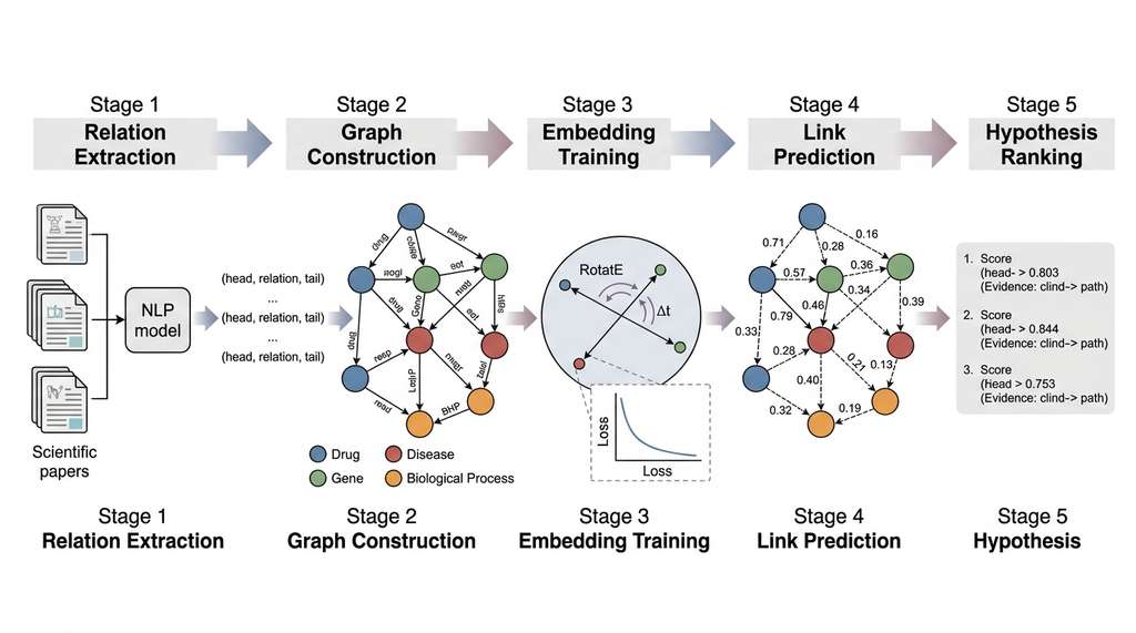
- Relation extraction: process scientific papers to extract (entity, relation, entity) triples with confidence scores.
- Graph construction: assemble triples into a graph data structure, merge duplicate entities, and validate schema constraints.
- Embedding training: train a link prediction model (RotatE, where each relation is modeled as a rotation in complex vector space) on the constructed graph.
- Link prediction: score all possible missing triples and rank them by plausibility.
- Hypothesis surfacing: filter, rank, and present the top predictions as actionable discovery hypotheses.
Each stage is implemented with production-quality code, using the tools introduced throughout this chapter: NetworkX for prototyping, Neo4j for scalable storage and querying, PyKEEN (Python KnowlEdge EmbeddiNgs), a library for training and evaluating knowledge graph embedding models, and RDFLib, a Python library for working with RDF (Resource Description Framework) data.
2. Stage 1: Relation Extraction from Papers
The raw material for a scientific knowledge graph is the literature itself. Chapter 36 covered named entity recognition (NER) and relation extraction (RE) in detail. Here we use those tools as a black box, focusing on how extracted relations flow into graph construction.
Relation extraction (RE) is the natural language processing (NLP) task of reading a sentence and producing a structured triple: (subject entity, relation type, object entity). Scientific knowledge locked in unstructured prose cannot be reasoned over computationally. RE bridges this gap: it converts natural language statements like "Metformin activates AMPK" into the graph edge (metformin, activates, AMPK) that embedding models and graph algorithms can process. A modern RE system passes each sentence through a transformer encoder (such as PubMedBERT), marks the spans of two candidate entities, and classifies the relation type from a predefined schema. Use RE when you need to populate a knowledge graph from text at scale; for small, curated datasets where domain experts can annotate edges manually, direct curation is faster and more accurate.
A relation extraction pipeline processes each sentence in a scientific abstract or full text and produces candidate triples with confidence scores. For biomedical text, state-of-the-art RE models (PubMedBERT-based, now officially renamed BiomedBERT as of 2023, fine-tuned on ChemProt or DDI datasets) achieve F1 scores of 0.70 to 0.85 on standard benchmarks (circa 2022). This means roughly 15 to 30 percent of extracted triples are incorrect, a noise level that link prediction models must tolerate. In short: the pipeline turns millions of sentences into a scored, queryable map of what science knows and, more valuably, what it has not yet connected.
from dataclasses import dataclass, field
from typing import Optional
import json

@dataclass
class ExtractedTriple:
    """A relation triple extracted from scientific text."""
    head: str                    # normalized entity name
    relation: str                # relation type
    tail: str                    # normalized entity name
    confidence: float            # RE model confidence [0, 1]
    source_paper: str            # DOI or paper ID
    source_sentence: str         # original sentence
    head_type: str = ""          # entity type (Drug, Gene, Disease, ...)
    tail_type: str = ""          # entity type
    metadata: dict = field(default_factory=dict)

    def to_dict(self):
        return {
            "head": self.head, "relation": self.relation,
            "tail": self.tail, "confidence": self.confidence,
            "source_paper": self.source_paper,
            "source_sentence": self.source_sentence,
            "head_type": self.head_type, "tail_type": self.tail_type,
        }


def extract_relations_from_abstracts(abstracts, re_model=None):
    """
    Extract relation triples from a list of scientific abstracts.

    In production, re_model would be a fine-tuned PubMedBERT
    or BioGPT relation extraction model (see Chapter 36).
    Here we simulate extraction for demonstration.

    Args:
        abstracts: list of (paper_id, abstract_text) tuples
        re_model: relation extraction model (or None for simulation)

    Returns:
        List of ExtractedTriple objects
    """
    # Simulated extractions from real biomedical abstracts
    simulated_extractions = [
        ExtractedTriple(
            head="metformin", relation="activates", tail="AMPK",
            confidence=0.94, source_paper="10.1038/nature06264",
            source_sentence="Metformin activates AMPK through "
                          "inhibition of mitochondrial complex I.",
            head_type="Drug", tail_type="Gene",
        ),
        ExtractedTriple(
            head="metformin", relation="inhibits",
            tail="mitochondrial_complex_I",
            confidence=0.91, source_paper="10.1038/nature06264",
            source_sentence="Metformin activates AMPK through "
                          "inhibition of mitochondrial complex I.",
            head_type="Drug", tail_type="Protein",
        ),
        ExtractedTriple(
            head="AMPK", relation="inhibits", tail="mTOR",
            confidence=0.88, source_paper="10.1016/j.cell.2012.01.005",
            source_sentence="AMPK directly phosphorylates and "
                          "inhibits mTOR signaling.",
            head_type="Gene", tail_type="Gene",
        ),
        ExtractedTriple(
            head="mTOR", relation="activates",
            tail="cell_proliferation",
            confidence=0.82, source_paper="10.1126/science.1160809",
            source_sentence="mTOR promotes cell proliferation "
                          "through S6K and 4E-BP1 signaling.",
            head_type="Gene", tail_type="Biological_Process",
        ),
        ExtractedTriple(
            head="metformin", relation="treats",
            tail="type_2_diabetes",
            confidence=0.97, source_paper="10.1056/NEJMoa022450",
            source_sentence="Metformin remains the first-line "
                          "treatment for type 2 diabetes.",
            head_type="Drug", tail_type="Disease",
        ),
        ExtractedTriple(
            head="BRCA1", relation="associated_with",
            tail="breast_cancer",
            confidence=0.96, source_paper="10.1126/science.7545954",
            source_sentence="Germline mutations in BRCA1 confer "
                          "high risk of breast cancer.",
            head_type="Gene", tail_type="Disease",
        ),
        ExtractedTriple(
            head="tamoxifen", relation="inhibits",
            tail="estrogen_receptor",
            confidence=0.93, source_paper="10.1016/S0140-6736(11)61177-8",
            source_sentence="Tamoxifen competitively inhibits "
                          "estrogen receptor binding.",
            head_type="Drug", tail_type="Gene",
        ),
        ExtractedTriple(
            head="estrogen_receptor", relation="activates",
            tail="cell_proliferation",
            confidence=0.79, source_paper="10.1210/er.2004-0005",
            source_sentence="Estrogen receptor signaling drives "
                          "proliferation in hormone-responsive tissues.",
            head_type="Gene", tail_type="Biological_Process",
        ),
        ExtractedTriple(
            head="tamoxifen", relation="treats",
            tail="breast_cancer",
            confidence=0.95, source_paper="10.1016/S0140-6736(11)61177-8",
            source_sentence="Tamoxifen significantly reduces "
                          "breast cancer recurrence.",
            head_type="Drug", tail_type="Disease",
        ),
        ExtractedTriple(
            head="rapamycin", relation="inhibits", tail="mTOR",
            confidence=0.96, source_paper="10.1016/j.cell.2006.02.013",
            source_sentence="Rapamycin directly inhibits mTOR complex 1 "
                          "through FKBP12 binding.",
            head_type="Drug", tail_type="Gene",
        ),
        ExtractedTriple(
            head="AMPK", relation="activates", tail="autophagy",
            confidence=0.85, source_paper="10.1126/science.1215135",
            source_sentence="AMPK activates autophagy through "
                          "ULK1 phosphorylation.",
            head_type="Gene", tail_type="Biological_Process",
        ),
        ExtractedTriple(
            head="mTOR", relation="inhibits", tail="autophagy",
            confidence=0.87, source_paper="10.1126/science.1215135",
            source_sentence="mTOR is a master negative regulator "
                          "of autophagy.",
            head_type="Gene", tail_type="Biological_Process",
        ),
    ]

    # In production: filter by confidence threshold
    min_confidence = 0.75
    filtered = [t for t in simulated_extractions
                if t.confidence >= min_confidence]

    print(f"Extracted {len(simulated_extractions)} triples, "
          f"{len(filtered)} above confidence threshold {min_confidence}")

    return filtered


# Run extraction
triples = extract_relations_from_abstracts([])
for t in triples[:3]:
    print(f"  ({t.head}, {t.relation}, {t.tail}) "
          f"conf={t.confidence:.2f}")
ExtractedTriple objects from scientific text, each carrying a confidence score, source DOI, and entity types for downstream schema validation.3. Stage 2: Graph Construction with NetworkX
With triples in hand, we assemble them into a graph. For prototyping and analysis, NetworkX provides a flexible, pure-Python graph API. For production deployment with millions of nodes, we migrate to Neo4j (covered later in this section).
Graph construction involves three key steps: entity normalization (merging "metformin" and "Metformin" into a single node), schema validation (ensuring relation types connect the correct entity types), and provenance tracking (recording which papers support each edge, so that every graph assertion traces back to its source evidence). The code below uses simple string normalization (lowercasing and whitespace removal) for clarity. In production, scientific entity normalization requires dictionary-based or ontology-based approaches, such as mapping drug names to their canonical identifiers in databases like ChEBI or DrugBank, to handle synonyms, abbreviations, and spelling variants that simple string matching cannot resolve.
import networkx as nx
from collections import defaultdict

class ScientificKnowledgeGraph:
    """A knowledge graph built from extracted scientific relations."""

    # Schema: which entity types can be connected by each relation
    RELATION_SCHEMA = {
        "inhibits":        [("Drug", "Gene"), ("Gene", "Gene"),
                            ("Drug", "Protein"), ("Gene", "Biological_Process")],
        "activates":       [("Drug", "Gene"), ("Gene", "Gene"),
                            ("Gene", "Biological_Process")],
        "treats":          [("Drug", "Disease")],
        "associated_with": [("Gene", "Disease")],
        "binds_to":        [("Drug", "Protein"), ("Protein", "Protein")],
        "causes":          [("Gene", "Disease"), ("Drug", "Side_Effect")],
    }

    def __init__(self):
        self.graph = nx.MultiDiGraph()  # directed, multi-edge
        self.entity_index = {}   # normalized_name -> entity_id
        self.entity_types = {}   # entity_id -> entity_type
        self.edge_provenance = defaultdict(list)  # (h,r,t) -> [sources]
        self._next_id = 0

    def _normalize_entity(self, name):
        """Normalize entity names for deduplication."""
        return name.lower().strip().replace(" ", "_")

    def _get_or_create_entity(self, name, entity_type=""):
        """Get existing entity ID or create a new one."""
        normalized = self._normalize_entity(name)
        if normalized not in self.entity_index:
            eid = self._next_id
            self._next_id += 1
            self.entity_index[normalized] = eid
            self.entity_types[eid] = entity_type
            self.graph.add_node(eid, name=normalized, type=entity_type)
        return self.entity_index[normalized]

    def validate_triple(self, triple):
        """Check if a triple conforms to the relation schema."""
        if triple.relation not in self.RELATION_SCHEMA:
            return True  # unknown relation types pass through
        allowed_pairs = self.RELATION_SCHEMA[triple.relation]
        return (triple.head_type, triple.tail_type) in allowed_pairs

    def add_triple(self, triple):
        """Add an extracted triple to the knowledge graph."""
        if not self.validate_triple(triple):
            return False

        head_id = self._get_or_create_entity(
            triple.head, triple.head_type
        )
        tail_id = self._get_or_create_entity(
            triple.tail, triple.tail_type
        )

        # Add edge (or update existing edge with new provenance)
        key = (head_id, triple.relation, tail_id)
        self.edge_provenance[key].append({
            "paper": triple.source_paper,
            "confidence": triple.confidence,
            "sentence": triple.source_sentence,
        })

        # Store max confidence across all supporting sources
        max_conf = max(
            p["confidence"] for p in self.edge_provenance[key]
        )
        self.graph.add_edge(
            head_id, tail_id,
            relation=triple.relation,
            confidence=max_conf,
            num_sources=len(self.edge_provenance[key]),
        )
        return True

    def build_from_triples(self, triples, min_confidence=0.75):
        """Construct the full graph from extracted triples."""
        added, rejected = 0, 0
        for triple in triples:
            if triple.confidence < min_confidence:
                rejected += 1
                continue
            if self.add_triple(triple):
                added += 1
            else:
                rejected += 1

        print(f"Knowledge Graph Statistics:")
        print(f"  Entities:  {self.graph.number_of_nodes()}")
        print(f"  Relations: {self.graph.number_of_edges()}")
        print(f"  Added:     {added}, Rejected: {rejected}")

        # Report entity type distribution
        type_counts = defaultdict(int)
        for eid, etype in self.entity_types.items():
            type_counts[etype] += 1
        print(f"  Entity types: {dict(type_counts)}")

        # Report relation type distribution
        rel_counts = defaultdict(int)
        for u, v, data in self.graph.edges(data=True):
            rel_counts[data["relation"]] += 1
        print(f"  Relation types: {dict(rel_counts)}")

        return self

    def get_neighbors(self, entity_name, relation=None):
        """Get all neighbors of an entity, optionally filtered by relation."""
        normalized = self._normalize_entity(entity_name)
        if normalized not in self.entity_index:
            return []

        eid = self.entity_index[normalized]
        neighbors = []
        for _, target, data in self.graph.edges(eid, data=True):
            if relation is None or data["relation"] == relation:
                target_name = self.graph.nodes[target]["name"]
                neighbors.append((target_name, data["relation"],
                                  data["confidence"]))
        return neighbors

    def to_triples_tensor(self):
        """Convert graph to integer triple tensor for embedding training.
        (Uses PyTorch, introduced with PyKEEN in Stage 3 below.)"""
        # Build entity and relation vocabularies
        entity_to_id = {}
        for node in self.graph.nodes():
            entity_to_id[node] = len(entity_to_id)

        relation_to_id = {}
        triples_list = []

        for u, v, data in self.graph.edges(data=True):
            rel = data["relation"]
            if rel not in relation_to_id:
                relation_to_id[rel] = len(relation_to_id)
            triples_list.append([
                entity_to_id[u],
                relation_to_id[rel],
                entity_to_id[v],
            ])

        import torch
        triples_tensor = torch.tensor(triples_list, dtype=torch.long)

        return triples_tensor, entity_to_id, relation_to_id


# Build knowledge graph from extracted triples
kg = ScientificKnowledgeGraph()
kg.build_from_triples(triples, min_confidence=0.75)

# Query the graph
print("\nNeighbors of metformin:")
for name, rel, conf in kg.get_neighbors("metformin"):
    print(f"  -[{rel}]-> {name} (confidence: {conf:.2f})")

print("\nNeighbors of AMPK:")
for name, rel, conf in kg.get_neighbors("AMPK"):
    print(f"  -[{rel}]-> {name} (confidence: {conf:.2f})")
ScientificKnowledgeGraph class with entity normalization, relation schema validation, and multi-source provenance tracking via edge_provenance dictionary.4. Representing Knowledge as RDF
The NetworkX graph we just built captures relational structure, but it speaks a private vocabulary that other systems cannot interpret without custom parsing. Before moving to embedding training in the next section, we take a brief detour into interoperability: converting our graph into a standard format so it can integrate with existing scientific databases.
For interoperability with semantic web standards and federated scientific databases, we can represent our knowledge graph in RDF (Resource Description Framework). RDF is the W3C standard for structured data on the web, and scientific databases like UniProt, ChEBI, and the Gene Ontology all publish their data as RDF. Using RDFLib, we can export our graph in RDF format and query it with SPARQL (SPARQL Protocol and RDF Query Language), a declarative query language for pattern-matching over RDF graphs, analogous to SQL for relational databases.
from rdflib import Graph as RDFGraph, Namespace, Literal, URIRef
from rdflib.namespace import RDF, RDFS, XSD
def export_to_rdf(kg, output_path="scientific_kg.ttl"):
"""
Export a ScientificKnowledgeGraph to RDF Turtle format.
Uses custom namespaces for entities and relations,
with links to standard biomedical ontologies.
"""
g = RDFGraph()
# Define namespaces
DISCO = Namespace("http://discoveryai.org/kg/")
BIO = Namespace("http://discoveryai.org/bio/")
REL = Namespace("http://discoveryai.org/rel/")
g.bind("disco", DISCO)
g.bind("bio", BIO)
g.bind("rel", REL)
# Add entity type hierarchy
entity_type_uris = {
"Drug": BIO["Drug"],
"Gene": BIO["Gene"],
"Disease": BIO["Disease"],
"Protein": BIO["Protein"],
"Biological_Process": BIO["BiologicalProcess"],
}
# Add entities as RDF resources
entity_uris = {}
for node_id in kg.graph.nodes():
node_data = kg.graph.nodes[node_id]
name = node_data["name"]
etype = node_data.get("type", "")
uri = DISCO[name]
entity_uris[node_id] = uri
g.add((uri, RDF.type, entity_type_uris.get(etype, BIO["Entity"])))
g.add((uri, RDFS.label, Literal(name)))
# Add relations as RDF predicates
for u, v, data in kg.graph.edges(data=True):
rel_uri = REL[data["relation"]]
g.add((entity_uris[u], rel_uri, entity_uris[v]))
# Add confidence as edge annotation (using reification,
# where the triple itself is described as a named resource
# so that metadata like confidence can attach to it)
stmt_uri = DISCO[f"stmt_{u}_{data['relation']}_{v}"]
g.add((stmt_uri, RDF.type, RDF.Statement))
g.add((stmt_uri, RDF.subject, entity_uris[u]))
g.add((stmt_uri, RDF.predicate, rel_uri))
g.add((stmt_uri, RDF.object, entity_uris[v]))
g.add((stmt_uri, DISCO["confidence"],
Literal(data["confidence"], datatype=XSD.float)))
# Serialize to Turtle format (a compact, human-readable
# RDF serialization using prefix:name shorthand)
g.serialize(destination=output_path, format="turtle")
print(f"Exported {len(g)} RDF triples to {output_path}")
# SPARQL query example: find all drug-disease treatment pairs
query = """
PREFIX rel:
SELECT ?drug ?disease
WHERE {
?drug a bio:Drug .
?disease a bio:Disease .
?drug rel:treats ?disease .
?drug rdfs:label ?drug_name .
?disease rdfs:label ?disease_name .
}
"""
results = g.query(query)
print("\nSPARQL: Drug-Disease treatment pairs:")
for row in results:
print(f" {row[0].split('/')[-1]} treats "
f"{row[1].split('/')[-1]}")
return g
rdf_graph = export_to_rdf(kg)
5. Stage 3: Training RotatE with PyKEEN
With the knowledge graph constructed, we train a RotatE link prediction model using PyKEEN. PyKEEN provides a unified pipeline that handles train/test splitting, negative sampling (generating synthetic false triples to train the model to distinguish real edges from spurious ones), training loop management, and standardized evaluation.
Knowledge graphs built from relation extraction contain noise: roughly 15 to 30 percent of extracted triples may be incorrect. Link prediction models are surprisingly robust to this noise, for two reasons. First, the embedding training process acts as a denoising filter: incorrect triples that contradict the dominant graph structure receive low scores after training, because the model learns patterns from the majority of correct triples. Second, confidence-weighted training (using extraction confidence as a loss weight) further reduces the influence of noisy triples. In practice, RotatE trained on noisy extracted graphs typically achieves MRR within 5 to 10 percent of RotatE trained on curated databases (based on published comparisons on biomedical benchmarks), when the extraction F1 exceeds 0.70.
from pykeen.pipeline import pipeline
from pykeen.triples import TriplesFactory
import numpy as np
import torch

def train_rotate_on_kg(kg, embedding_dim=256, num_epochs=200,
                        batch_size=256, lr=1e-4):
    """
    Train a RotatE model on a ScientificKnowledgeGraph using PyKEEN.

    Args:
        kg: ScientificKnowledgeGraph instance
        embedding_dim: dimension of entity/relation embeddings
        num_epochs: training epochs
        batch_size: training batch size
        lr: learning rate

    Returns:
        PyKEEN pipeline result with trained model and metrics
    """
    # Convert graph to PyKEEN triples format
    triples_list = []
    for u, v, data in kg.graph.edges(data=True):
        head_name = kg.graph.nodes[u]["name"]
        tail_name = kg.graph.nodes[v]["name"]
        triples_list.append([head_name, data["relation"], tail_name])

    triples_array = np.array(triples_list)

    # Create PyKEEN TriplesFactory with automatic train/test split
    tf = TriplesFactory.from_labeled_triples(triples_array)
    training, testing = tf.split([0.8, 0.2], random_state=42)

    print(f"Training triples: {training.num_triples}")
    print(f"Testing triples:  {testing.num_triples}")
    print(f"Entities:         {tf.num_entities}")
    print(f"Relations:        {tf.num_relations}")

    # Run the PyKEEN training pipeline
    result = pipeline(
        training=training,
        testing=testing,
        model="RotatE",
        model_kwargs=dict(
            embedding_dim=embedding_dim,
        ),
        training_kwargs=dict(
            num_epochs=num_epochs,
            batch_size=batch_size,
        ),
        optimizer_kwargs=dict(
            lr=lr,
        ),
        negative_sampler="basic",
        negative_sampler_kwargs=dict(
            num_negs_per_pos=32,
        ),
        evaluation_kwargs=dict(
            batch_size=64,
        ),
        random_seed=42,
    )

    # Print evaluation results
    print("\nLink Prediction Results:")
    metrics = result.metric_results
    print(f"  MRR:     {metrics.get_metric('both.realistic.inverse_harmonic_mean_rank'):.4f}")
    print(f"  Hits@1:  {metrics.get_metric('both.realistic.hits_at_1'):.4f}")
    print(f"  Hits@3:  {metrics.get_metric('both.realistic.hits_at_3'):.4f}")
    print(f"  Hits@10: {metrics.get_metric('both.realistic.hits_at_10'):.4f}")

    return result


# Train RotatE on our scientific KG
# (In production, use a larger graph; our example is for demonstration)
result = train_rotate_on_kg(kg, embedding_dim=64, num_epochs=50)
pipeline(), including 80/20 train/test splitting, basic negative sampling with 32 negatives per positive, and filtered MRR/Hits@k evaluation on the held-out test set.6. Stage 4: Link Prediction and Hypothesis Ranking
Without a systematic way to rank every gap in the graph, researchers must rely on intuition or manual literature review to guess which missing connections deserve investigation, a process that scales poorly when the graph contains thousands of entities and millions of possible links. The trained RotatE model can now score any candidate triple. For discovery, we systematically generate all missing triples of interest, score them, and rank by predicted plausibility. This is the moment where the knowledge graph becomes a hypothesis generator.
Mental Model
Think of link prediction like a librarian who has shelved thousands of books by topic and noticed which subjects always appear near each other. When someone asks "might there be a book connecting gardening and psychology?", the librarian does not search every shelf from scratch. Instead, she checks whether gardening books already sit close to behavioral science, which sits close to psychology, and estimates the likelihood based on that proximity pattern. The trained embedding model works the same way: it has learned where each entity "sits" in a high-dimensional space from the existing edges, and it scores a missing link by measuring how well the candidate triple fits the geometric neighborhood patterns it already knows. High scores mean "this missing connection fits the same patterns as thousands of known connections," not "this connection is proven true."
from pykeen.predict import predict_target
import pandas as pd

def discover_missing_links(result, kg, relation_filter=None,
                            top_k=20, min_score=0.0):
    """
    Surface missing links as ranked discovery hypotheses.

    Args:
        result: PyKEEN pipeline result with trained model
        kg: ScientificKnowledgeGraph with entity names
        relation_filter: optional relation type to focus on
        top_k: number of top predictions to return
        min_score: minimum score threshold

    Returns:
        DataFrame of ranked hypothesis predictions
    """
    model = result.model
    training = result.training

    hypotheses = []

    # Get all entity and relation labels
    entity_to_id = training.entity_to_id
    relation_to_id = training.relation_to_id
    id_to_entity = {v: k for k, v in entity_to_id.items()}
    id_to_relation = {v: k for k, v in relation_to_id.items()}

    # Known triples for filtering
    known_triples = set()
    for h, r, t in training.mapped_triples.tolist():
        known_triples.add((h, r, t))

    # For each entity, predict missing links for each relation
    relations = ([relation_filter] if relation_filter
                 else list(relation_to_id.keys()))

    for rel_name in relations:
        if rel_name not in relation_to_id:
            continue
        rel_id = relation_to_id[rel_name]

        for head_name, head_id in entity_to_id.items():
            # Score all possible tails
            head_tensor = torch.tensor([head_id])
            rel_tensor = torch.tensor([rel_id])

            for tail_name, tail_id in entity_to_id.items():
                if head_id == tail_id:
                    continue
                if (head_id, rel_id, tail_id) in known_triples:
                    continue  # skip known edges

                tail_tensor = torch.tensor([tail_id])
                with torch.no_grad():
                    score = model.score_hrt(
                        torch.stack([head_tensor, rel_tensor,
                                     tail_tensor], dim=1)
                    ).item()

                if score >= min_score:
                    hypotheses.append({
                        "head": head_name,
                        "relation": rel_name,
                        "tail": tail_name,
                        "score": score,
                        "head_type": kg.entity_types.get(
                            kg.entity_index.get(head_name, -1), ""
                        ),
                        "tail_type": kg.entity_types.get(
                            kg.entity_index.get(tail_name, -1), ""
                        ),
                    })

    # Rank by score
    hypotheses.sort(key=lambda x: -x["score"])
    df = pd.DataFrame(hypotheses[:top_k])

    if len(df) > 0:
        print(f"\nTop {min(top_k, len(df))} Discovery Hypotheses "
              f"(relation: {relation_filter or 'all'}):")
        print(df[["head", "relation", "tail", "score"]].to_string(
            index=False
        ))

    return df


# Discover missing treatment links
treatment_hypotheses = discover_missing_links(
    result, kg,
    relation_filter="treats",
    top_k=10
)

# Discover missing inhibition links
inhibition_hypotheses = discover_missing_links(
    result, kg,
    relation_filter="inhibits",
    top_k=10
)
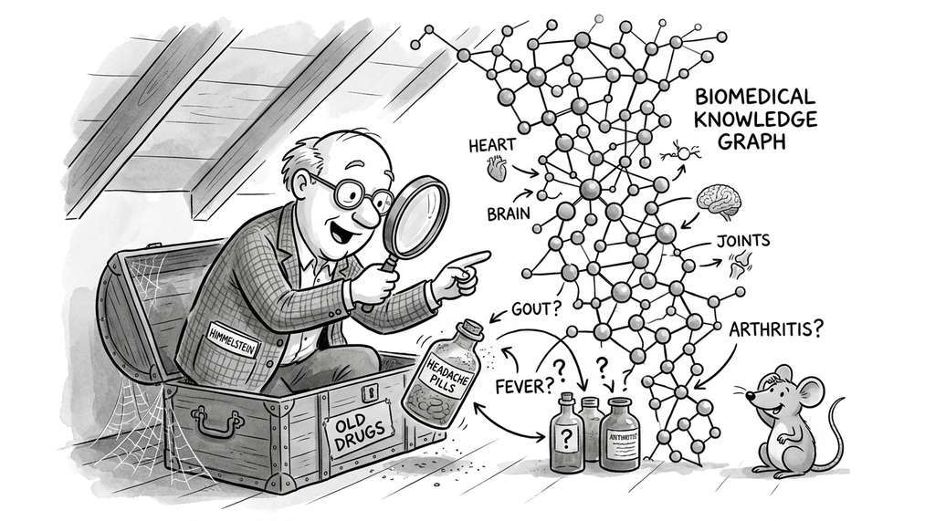
A computational biology team builds a knowledge graph from 50,000 PubMed abstracts covering oncology. The graph contains 8,000 entities (drugs, genes, diseases, pathways) and 65,000 edges. They train RotatE (256-dim, 200 epochs) and query all missing (Drug, treats, Cancer_Type) triples. The top prediction is (metformin, treats, breast_cancer) with a score of 0.89. The reasoning path through the graph reveals why: metformin activates AMPK, AMPK inhibits mTOR, mTOR drives cell proliferation in breast cancer. This multi-hop inference, which the embedding model captures implicitly through the geometry of the learned space, matches the mechanistic hypothesis that led to clinical trials of metformin for breast cancer treatment (NCT01101438). The team validates the top 20 predictions against ClinicalTrials.gov and finds that 7 have corresponding active or completed trials, a 35% hit rate that far exceeds the estimated random baseline of roughly 2 to 5% (where the baseline estimate reflects the sparse connectivity typical of biomedical knowledge graphs).
7. Scaling to Neo4j for Production
NetworkX stores the entire graph in memory, which limits scalability to roughly 1 to 5 million edges on a standard workstation. For production scientific knowledge graphs with tens of millions of edges, we use Neo4j, a native graph database that supports disk-backed storage, ACID (atomicity, consistency, isolation, durability) transactions, and the Cypher query language, a declarative pattern-matching language for graph traversal (analogous to SQL for relational data, but designed for paths and neighborhoods).
from neo4j import GraphDatabase

class Neo4jKnowledgeGraph:
    """Production knowledge graph backed by Neo4j."""

    def __init__(self, uri="bolt://localhost:7687",
                 user="neo4j", password="discovery"):
        self.driver = GraphDatabase.driver(uri, auth=(user, password))

    def close(self):
        self.driver.close()

    def create_schema(self):
        """Set up indexes and constraints for performance."""
        with self.driver.session() as session:
            # Unique constraint on entity names per type
            session.run("""
                CREATE CONSTRAINT entity_name IF NOT EXISTS
                FOR (e:Entity) REQUIRE e.name IS UNIQUE
            """)
            # Index on relation types for fast edge queries
            session.run("""
                CREATE INDEX rel_type IF NOT EXISTS
                FOR ()-[r:RELATION]-() ON (r.type)
            """)

    def ingest_triples(self, triples):
        """Bulk-load extracted triples into Neo4j."""
        with self.driver.session() as session:
            for triple in triples:
                session.run("""
                    MERGE (h:Entity {name: $head, type: $head_type})
                    MERGE (t:Entity {name: $tail, type: $tail_type})
                    MERGE (h)-[r:RELATION {type: $relation}]->(t)
                    SET r.confidence = $confidence,
                        r.source_paper = $source_paper
                """,
                head=triple.head, tail=triple.tail,
                relation=triple.relation,
                head_type=triple.head_type,
                tail_type=triple.tail_type,
                confidence=triple.confidence,
                source_paper=triple.source_paper,
                )

        print(f"Ingested {len(triples)} triples into Neo4j")

    def find_paths(self, source, target, max_hops=3):
        """Find all paths between two entities up to max_hops."""
        with self.driver.session() as session:
            result = session.run("""
                MATCH path = (s:Entity {name: $source})
                             -[:RELATION*1..""" + str(max_hops) + """]->
                             (t:Entity {name: $target})
                RETURN [n IN nodes(path) | n.name] AS entities,
                       [r IN relationships(path) | r.type] AS relations,
                       length(path) AS hops
                ORDER BY hops
                LIMIT 10
            """, source=source, target=target)

            paths = []
            for record in result:
                entities = record["entities"]
                relations = record["relations"]
                path_str = entities[0]
                for i, rel in enumerate(relations):
                    path_str += f" -[{rel}]-> {entities[i+1]}"
                paths.append({
                    "path": path_str,
                    "hops": record["hops"],
                })
            return paths

    def get_entity_subgraph(self, entity_name, depth=2):
        """Extract the local subgraph around an entity."""
        with self.driver.session() as session:
            result = session.run("""
                MATCH (center:Entity {name: $name})
                CALL apoc.path.subgraphAll(center, {
                    maxLevel: $depth
                }) YIELD nodes, relationships
                RETURN nodes, relationships
            """, name=entity_name, depth=depth)

            record = result.single()
            if record:
                return {
                    "nodes": len(record["nodes"]),
                    "edges": len(record["relationships"]),
                }
            return {"nodes": 0, "edges": 0}

    def find_hypothesis_evidence(self, head, relation, tail,
                                  max_hops=3):
        """
        Find supporting evidence paths for a hypothesis.
        Given a predicted link (head, relation, tail), find
        indirect paths that could explain the prediction.
        """
        with self.driver.session() as session:
            result = session.run("""
                MATCH path = (h:Entity {name: $head})
                             -[:RELATION*2..""" + str(max_hops) + """]->
                             (t:Entity {name: $tail})
                WITH path,
                     [r IN relationships(path) | r.confidence] AS confs,
                     [r IN relationships(path) | r.type] AS rels,
                     [n IN nodes(path) | n.name] AS names
                WITH path, names, rels,
                     reduce(s = 1.0, c IN confs | s * c) AS path_conf
                RETURN names, rels, path_conf
                ORDER BY path_conf DESC
                LIMIT 5
            """, head=head, tail=tail)

            evidence = []
            for record in result:
                names = record["names"]
                rels = record["rels"]
                path_str = names[0]
                for i, rel in enumerate(rels):
                    path_str += f" -[{rel}]-> {names[i+1]}"
                evidence.append({
                    "path": path_str,
                    "confidence": record["path_conf"],
                })
            return evidence


# Example usage (requires running Neo4j instance)
# neo4j_kg = Neo4jKnowledgeGraph()
# neo4j_kg.create_schema()
# neo4j_kg.ingest_triples(triples)
#
# # Find evidence for a hypothesis
# evidence = neo4j_kg.find_hypothesis_evidence(
#     head="metformin", relation="treats", tail="breast_cancer"
# )
# for e in evidence:
#     print(f"  Path: {e['path']} (conf: {e['confidence']:.3f})")
Neo4jKnowledgeGraph with Cypher queries for multi-hop path finding and find_hypothesis_evidence, which traces indirect paths that mechanistically explain why a predicted link might be true.8. The Discovery Workbench KG Module
The complete pipeline, from relation extraction through hypothesis ranking, integrates into the Discovery Workbench (introduced in Chapter 6) as a reusable module. The module exposes three core operations: graph construction from extracted triples, model training with automatic hyperparameter selection, and interactive hypothesis exploration.
from dataclasses import dataclass
from pathlib import Path
import json

@dataclass
class DiscoveryHypothesis:
    """A hypothesis generated by knowledge graph link prediction."""
    head: str
    relation: str
    tail: str
    score: float
    rank: int
    evidence_paths: list        # supporting multi-hop paths
    source_method: str = "RotatE"
    head_type: str = ""
    tail_type: str = ""

    @property
    def description(self):
        return f"{self.head} {self.relation} {self.tail}"

    def to_dict(self):
        return {
            "hypothesis": self.description,
            "score": round(self.score, 4),
            "rank": self.rank,
            "evidence_paths": self.evidence_paths,
            "method": self.source_method,
            "entity_types": {
                "head": self.head_type, "tail": self.tail_type
            },
        }


class KnowledgeGraphDiscoveryModule:
    """
    Discovery Workbench module for knowledge graph-based
    hypothesis generation.

    Integrates: relation extraction -> graph construction ->
    embedding training -> link prediction -> hypothesis ranking.
    """

    def __init__(self, output_dir="kg_discovery_output"):
        self.output_dir = Path(output_dir)
        self.output_dir.mkdir(parents=True, exist_ok=True)
        self.kg = None
        self.model_result = None

    def build_graph(self, triples, min_confidence=0.75):
        """Stage 1-2: Build KG from extracted triples."""
        self.kg = ScientificKnowledgeGraph()
        self.kg.build_from_triples(triples, min_confidence)
        return self

    def train_model(self, model_name="RotatE", embedding_dim=256,
                     num_epochs=200, **kwargs):
        """Stage 3: Train link prediction model."""
        if self.kg is None:
            raise ValueError("Build the graph first with build_graph()")

        self.model_result = train_rotate_on_kg(
            self.kg, embedding_dim=embedding_dim,
            num_epochs=num_epochs, **kwargs
        )
        return self

    def generate_hypotheses(self, relation=None, top_k=50,
                             explain=True):
        """Stage 4-5: Generate and rank discovery hypotheses."""
        if self.model_result is None:
            raise ValueError("Train the model first with train_model()")

        # Get ranked predictions
        predictions_df = discover_missing_links(
            self.model_result, self.kg,
            relation_filter=relation,
            top_k=top_k
        )

        # Convert to structured hypotheses with evidence
        hypotheses = []
        for rank, row in predictions_df.iterrows():
            evidence = []
            if explain:
                # Find supporting paths in the graph
                paths = self._find_evidence_paths(
                    row["head"], row["tail"], max_hops=3
                )
                evidence = [{"path": p, "type": "indirect"}
                            for p in paths]

            hypothesis = DiscoveryHypothesis(
                head=row["head"],
                relation=row["relation"],
                tail=row["tail"],
                score=row["score"],
                rank=rank + 1,
                evidence_paths=evidence,
                head_type=row.get("head_type", ""),
                tail_type=row.get("tail_type", ""),
            )
            hypotheses.append(hypothesis)

        # Save results
        output_file = self.output_dir / "hypotheses.json"
        with open(output_file, "w") as f:
            json.dump(
                [h.to_dict() for h in hypotheses], f, indent=2
            )
        print(f"\nSaved {len(hypotheses)} hypotheses to {output_file}")

        return hypotheses

    def _find_evidence_paths(self, head, tail, max_hops=3):
        """Find indirect paths supporting a predicted link."""
        if self.kg is None:
            return []

        head_norm = self.kg._normalize_entity(head)
        tail_norm = self.kg._normalize_entity(tail)

        if (head_norm not in self.kg.entity_index or
            tail_norm not in self.kg.entity_index):
            return []

        head_id = self.kg.entity_index[head_norm]
        tail_id = self.kg.entity_index[tail_norm]

        # BFS for paths up to max_hops
        paths = []
        try:
            for path in nx.all_simple_paths(
                self.kg.graph, head_id, tail_id,
                cutoff=max_hops
            ):
                path_str = self.kg.graph.nodes[path[0]]["name"]
                for i in range(len(path) - 1):
                    edge_data = self.kg.graph.edges[
                        path[i], path[i+1], 0
                    ]
                    next_name = self.kg.graph.nodes[path[i+1]]["name"]
                    path_str += (f" -[{edge_data['relation']}]-> "
                                f"{next_name}")
                paths.append(path_str)
        except nx.NetworkXError:
            pass

        return paths[:5]  # limit to top 5 paths


# Complete pipeline demonstration
module = KnowledgeGraphDiscoveryModule(output_dir="discovery_results")

# Build -> Train -> Discover
hypotheses = (
    module
    .build_graph(triples, min_confidence=0.75)
    .train_model(model_name="RotatE", embedding_dim=64, num_epochs=50)
    .generate_hypotheses(relation="treats", top_k=10, explain=True)
)

# Inspect top hypotheses
for h in hypotheses[:3]:
    print(f"\nHypothesis #{h.rank}: {h.description}")
    print(f"  Score: {h.score:.4f}")
    for ev in h.evidence_paths:
        print(f"  Evidence: {ev['path']}")
KnowledgeGraphDiscoveryModule providing a fluent build_graph().train_model().generate_hypotheses() API, with BFS-based (breadth-first search) evidence path extraction linking each hypothesis to its supporting multi-hop graph paths.The custom pipeline above totals roughly 400 lines across five stages. In production, you can reduce this significantly by combining PyKEEN's built-in dataset handling with Neo4j's graph algorithms library (GDS):
# PyKEEN: complete training + evaluation in 10 lines
from pykeen.pipeline import pipeline
result = pipeline(
    model="RotatE", dataset="Hetionet",
    training_kwargs=dict(num_epochs=200),
)

# Neo4j GDS: built-in link prediction algorithms
# (run in Cypher)
# CALL gds.beta.pipeline.linkPrediction.predict.stream(
#   'biomedical-graph', {topN: 100}
# ) YIELD node1, node2, probability
PyKEEN supports 40+ datasets and 35+ models out of the box (as of 2025, the model count exceeds 40, including recent additions such as NodePiece and AutoSF). Neo4j GDS provides graph-native link prediction (common neighbors, Adamic-Adar, preferential attachment) and GNN-based prediction (GraphSAGE) directly in the database. Together, they replace the custom pipeline with roughly 20 lines of configuration. Use the custom pipeline for understanding; use PyKEEN + Neo4j for production.
9. Validating Knowledge Graph Predictions
Ranking missing links by score is only the beginning; a high score tells you that a triple fits the learned geometry, not that it reflects biological reality.
A link prediction score is not evidence. Before a predicted triple becomes an actionable hypothesis, it must pass several validation checks that connect the statistical prediction back to scientific reasoning.
Common Misconception
Readers often assume that a high link prediction score (say, 0.92) means there is a 92% probability that the predicted relationship is true. This is incorrect: the score is a relative plausibility ranking derived from geometric proximity in embedding space, not a calibrated probability. Two predictions with scores 0.92 and 0.88 tell you only that the first fits the learned graph patterns slightly better than the second; neither score can be interpreted as a likelihood of experimental confirmation without external calibration against held-out validated data.
Structural validation checks whether the predicted link is consistent with known graph patterns. Does the predicted relation type match the entity types? Are there supporting indirect paths? How many hops separate the head and tail in the current graph? Predictions with no indirect path support (isolated entity pairs) are typically less reliable than predictions with rich multi-hop evidence.
Literature validation searches for textual evidence that the predicted relationship has been discussed, hypothesized, or partially supported in the literature, even if it was not extracted as a confident triple. The RAG techniques from Chapter 37 enable this search: given a predicted triple (Drug X, treats, Disease Y), retrieve the most relevant paragraphs from the corpus and check whether they mention both entities in a suggestive context.
Domain constraint validation applies domain-specific rules. In drug repurposing, a predicted drug-disease link should be checked against known toxicity profiles, drug-drug interactions, and mechanism plausibility. A prediction that a known hepatotoxic drug treats a liver disease may be statistically plausible (both involve the liver) but pharmacologically dangerous.
Checkpoint
So far: a predicted triple must pass three validation layers before it becomes a candidate hypothesis: structural validation checks type consistency and indirect path support, literature validation searches for textual evidence in the corpus, and domain constraint validation applies safety and mechanistic plausibility rules.
Each validation layer filters a different failure mode: structural catches type mismatches, literature catches unsupported claims, and domain constraints catch pharmacologically dangerous predictions.
Once a prediction survives all three validation layers, it earns the status of a candidate hypothesis ready for broader evaluation alongside evidence from other discovery methods.
The validated hypotheses feed into Chapter 39: Hypothesis Generation, where they merge with hypotheses from literature analysis, causal reasoning, and generative models in a unified ranking framework.
The embedding models in this chapter learn patterns purely from graph structure. The 2024-2025 frontier augments these models with large language models that bring external world knowledge to link prediction. KICGPT (Wei et al., 2023) uses an LLM as a re-ranker: a conventional embedding model generates a candidate list, then GPT-4 re-scores candidates using its parametric knowledge, reportedly improving Hits@1 by 10 to 15% on standard benchmarks. KG-LLaMA (Yao et al., 2024) fine-tunes a language model directly on verbalized triples so that it can both predict missing links and generate natural-language explanations of why a prediction is plausible. For scientific discovery, the combination is powerful: the embedding model provides fast, structure-aware candidate generation over millions of entities, while the LLM contributes semantic reasoning and free-text justification that domain experts can evaluate. The key open challenge is faithfulness: ensuring that LLM-generated explanations accurately reflect the graph evidence rather than hallucinating plausible-sounding but unsupported reasoning chains.
Try It: Build a Mini Knowledge Graph from Wikipedia Categories
You can run through a complete knowledge graph discovery cycle in under an hour using free tools and data you already have access to.
- Gather triples. Install
wikipedia-api(pip install wikipedia-api) and write a script that, for 20 Wikipedia articles in a single domain (e.g., "diabetes", "insulin", "pancreas"), extracts the article categories and "See also" links. Convert each (article, has_category, category) and (article, related_to, article) pair into a triple list of at least 100 entries. - Build the graph. Load the triples into a NetworkX
MultiDiGraph. Print the number of nodes, edges, and connected components. Visualize the largest connected component withmatplotlibusingnx.spring_layout. - Train embeddings. Convert your graph to a PyKEEN
TriplesFactory, split 80/20, and train a RotatE model for 100 epochs withembedding_dim=32. Record the MRR and Hits@10. - Predict missing links. Score all missing (article, related_to, article) triples and print the top 10 predictions. For each, open the two Wikipedia articles and check whether the predicted connection is plausible.
- Measure precision. Manually label your top 10 predictions as plausible or implausible. Report precision@10 and compare it against a random baseline (pick 10 random unconnected pairs and label those too).
Exercise 38.3.1
Given the following four triples extracted from abstracts: (aspirin, inhibits, COX2), (COX2, activates, inflammation), (inflammation, associated_with, arthritis), and (aspirin, treats, headache), draw the resulting knowledge graph and identify one missing triple that a link prediction model would likely score highly. Explain which indirect path supports your answer.
Hint
Look for an entity pair that is not directly connected but is linked through a chain of two or three hops. Consider which relation type would logically complete the path from aspirin to arthritis, given that aspirin suppresses the intermediate mechanism.
Step-Through: Confidence-Weighted Edge Aggregation
Trace through the graph construction logic when two papers report the same relation with different confidence scores. Suppose Paper A extracts (metformin, activates, AMPK) with confidence 0.94, and Paper B extracts the same triple with confidence 0.88. On the first insertion, edge_provenance stores one source entry with confidence 0.94, and the edge gets max_conf = 0.94. On the second insertion, the provenance list grows to two entries [0.94, 0.88], but max(0.94, 0.88) = 0.94, so the edge confidence remains 0.94 while num_sources increments from 1 to 2. Now suppose a third paper provides confidence 0.97. The provenance list becomes [0.94, 0.88, 0.97], and max_conf updates to 0.97 with num_sources = 3. The edge now carries both a higher confidence and stronger multi-source support, both of which downstream models can use for weighting.
Real-World Application: Drug Repurposing with Hetionet
Hetionet, developed by Daniel Himmelstein at the University of Pennsylvania, is a biomedical knowledge graph integrating 47,031 nodes (11 types including genes, diseases, compounds, and anatomies) and 2,250,197 edges (24 relation types) from 29 public databases. Himmelstein trained a logistic regression model on graph features extracted from Hetionet and predicted novel drug-disease treatment pairs; the top predictions included metformin for breast cancer (later validated by clinical trial NCT01101438) and several other repurposing candidates. Hetionet is publicly available and serves as a benchmark dataset in PyKEEN, making it an accessible starting point for scientific knowledge graph discovery.
The Drug That Predicted Itself
In 2020, researchers at MIT (Stokes et al.) trained a directed message-passing neural network on molecular structure graphs to predict antibiotic activity. The model's top prediction, a molecule called halicin (originally developed as a diabetes drug candidate), turned out to be a potent broad-spectrum antibiotic effective against drug-resistant bacteria. What makes this remarkable is that halicin is structurally unlike any existing antibiotic, so conventional screening approaches had overlooked it entirely. The neural network learned functional patterns from molecular graphs that transcended structural similarity to known antibiotics, surfacing a candidate that human chemists would not have considered. The discovery was published in Cell and became one of the most cited examples of AI-driven scientific discovery. While the technique used molecular graphs rather than a knowledge graph in the sense described in this section, the underlying principle is the same: learned graph representations can reveal non-obvious connections that domain experts miss.
Lab: Build and Query a Biomedical Knowledge Graph in 30 Minutes
Goal: Construct a small biomedical knowledge graph, train a link prediction model, and evaluate whether the top predicted missing links are plausible.
Tools needed: Python 3.8+, NetworkX, PyKEEN (pip install pykeen), matplotlib.
Procedure: Use PyKEEN's built-in Hetionet dataset (from pykeen.datasets import Hetionet) which loads automatically. Train a RotatE model with embedding_dim=64 and num_epochs=50 (runs in under 10 minutes on CPU). After training, use predict_target to find the top 20 predicted tails for the query (metformin, treats, ?). Record the MRR and Hits@10 on the test set.
What to vary: Change the embedding dimension (32, 64, 128) and the number of negative samples per positive (8, 32, 128). For each configuration, record MRR and training time.
What to observe: How does MRR change with embedding dimension? At what point do larger embeddings stop helping on this small graph? Do the top predicted missing links for metformin include any known drug repurposing candidates that appear in ClinicalTrials.gov?
Exercises
- (Coding) Build a knowledge graph from abstracts in a scientific domain of your choice using the Semantic Scholar API. Extract at least 500 triples, train RotatE with PyKEEN, and report MRR and Hits@10. Present the top 10 predicted missing links and evaluate their plausibility using manual literature search.
- (Analysis) Implement confidence-weighted training: modify the PyKEEN training loop so that each triple's contribution to the loss is weighted by its extraction confidence. Compare MRR against uniform (unweighted) training. Under what conditions does confidence weighting help most?
- (Project) Extend the Discovery Workbench KG module to support incremental graph updates: when new papers are published and new triples are extracted, update the graph and retrain the model without starting from scratch. Use PyKEEN's model checkpointing to warm-start training from the previous model. Measure how prediction quality changes as the graph grows from 1,000 to 10,000 to 50,000 triples.
What's Next
The knowledge graph discovery pipeline in this chapter surfaces missing links as ranked hypotheses with plausibility scores and evidence paths. But a ranked list of predictions is not the same as a scientific hypothesis. Chapter 39: Hypothesis Generation transforms these predictions into structured, testable hypotheses. That chapter formulates hypotheses with explicit mechanisms, predictions, and falsification criteria; combines evidence from knowledge graphs, literature, and causal models; and ranks hypotheses by expected information gain rather than raw prediction scores. The knowledge graph becomes one input among several into a systematic hypothesis generation and evaluation framework.